
In the past, we have authored blog posts covering a wide range of topics, including machine learning algorithms such as classification and prediction. Our intention has always been to assist you in enhancing your understanding of how machines operate. We invite you to explore our website and take a look at some of the articles we have published. We would greatly appreciate any feedback you might have, as it would tremendously aid us in refining our writing. Please feel free to follow the provided links to access some of our featured pieces.
In this blog post, our focus will be on comprehending the functioning of mathematical support vector machines. Furthermore, we will delve into the various categories of SVMs and provide insight into their practical implementation using the Python programming language. Without further ado, let’s commence our exploration.
Introduction
Support Vector Machine (SVM), among the most extensively applied supervised learning methods, serves a dual purpose by addressing both classification and regression challenges. Nevertheless, its predominant usage lies in the realm of Machine Learning Classification tasks.
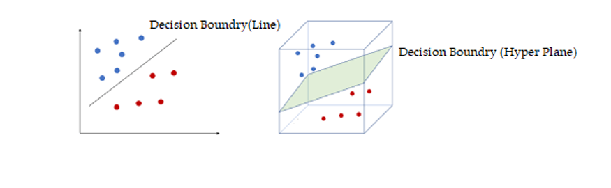
Upon receiving input data points, a support vector machine constructs a hyperplane – which, in two-dimensional space, translates to a line – meticulously partitioning the data points into two distinct groupings.
This demarcation, referred to as the decision boundary, constitutes the said line or hyperplane. Notably, data points situated on one side of this boundary align with one class, while those positioned on the opposite side align with a different class.
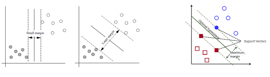
SVMs present two crucial advantages in contrast to more contemporary algorithms like neural networks: heightened computational speed and enhanced performance, particularly when dealing with a reduced sample size, often within the thousands. The data points nearest to the hyperplane, known as support vectors, hold sway over the positioning and orientation of the hyperplane itself. Various hyperplanes can potentially be employed to bifurcate the two classifications of data points.
Within the SVM algorithm, the hyperplane possessing the most extensive margin is selected as the optimal choice. This particular hyperplane is referred to as the Maximum Marginal Hyperplane (MMH). Imagining two planes, denoted as H1 and H2, which run parallel to the hyperplane of the decision boundary and traverse through the support vectors, they should maintain equal distance from the hyperplane.
The margin, in this context, signifies the separation between the H1 and H2 planes, underlining a critical aspect of SVM’s decision-making process.
Types of Support Machine
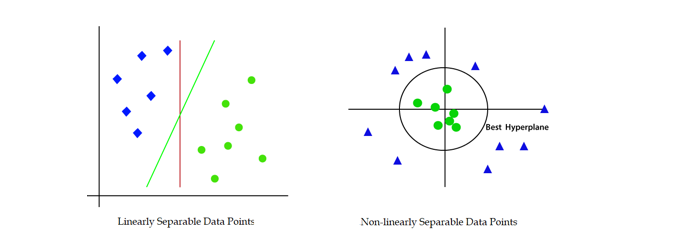
Support Vector Machines (SVM) come in two distinct variants: Linear SVM and Non-linear SVM.
The Linear SVM is harnessed for the classification of data points exhibiting linear separability. In contrast, the Non-linear SVM is employed when dealing with data points that showcase non-linear separability.
Non-linear SVM operates through the following consecutive steps:
-
It employs the kernel trick to transform low-dimensional data points into higher-dimensional counterparts that can be delineated using a linear approach.
-
Subsequently, a linear hyperplane is employed to categorize the transformed data points.
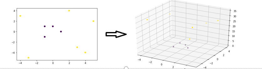
The kernel within SVM algorithms is a compilation of mathematical functions. These functions serve the purpose of transmuting non-linearly separable low-dimensional data points into high-dimensional ones that can be linearly separated. Prominent kernel functions encompass the Gaussian, Linear, Polynomial, Radial Basis Function (RBF), Sigmoid, among others.
Consider a scenario involving 2-dimensional data points that are not linearly separable. By introducing a third dimension defined as \(z = x^2 + y^2\), it becomes feasible to convert the initial data points into a configuration that allows linear separation to be applied.
Let’s demonstrate it by using one numerical example
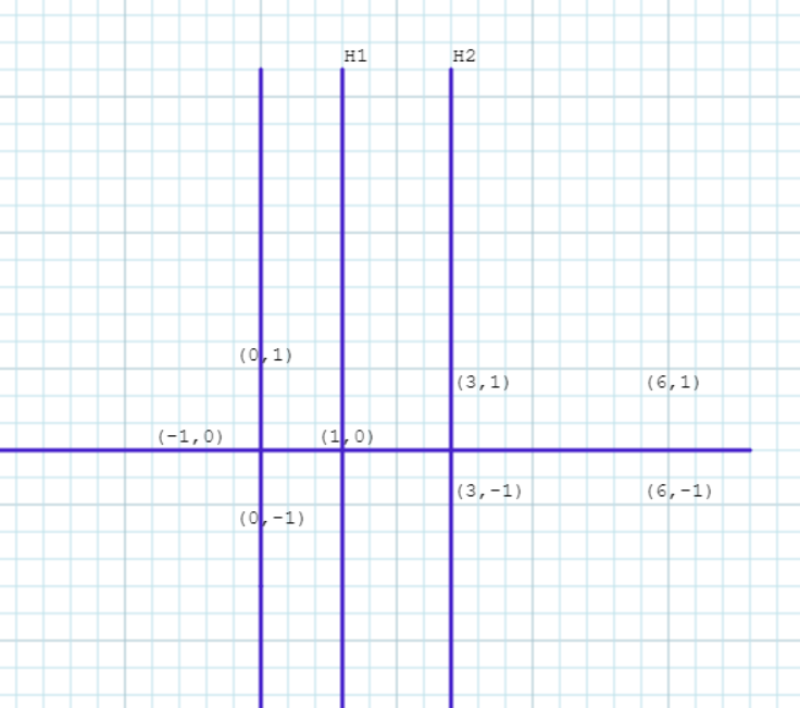
Example: Consider following data points
- Positively Labelled Data Points:(3,1),(3,-1),(6,1),(6,-1)
- Negatively Labelled Data Points:(1,0),(0,1),(0,-1),(-1,0)
Determine the equation of the hyperplane that divides the above data points into two classes. Then predict the class of data point (5,2).
Solution: First plot the given points
Positive Points: (3,1),(3,-1),(6,1),(6,-1)
Negative Points: (1,0),(0,1),(0,-1),(-1,0)
Support vectors are
s1=(1,0), s2=(3,1), s3=(3,-1)
Augment support vectors with bias = 1
s1=(1,0,1), s2=(3,1,1), s3=(3,-1,1)
Since there are three support vectors, we need to calculate three variables. Thus, three linear equations can be written as
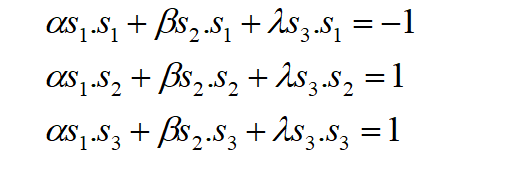
Because s1 belongs to the negative class and s2, s3, which are points belonging to the positive class, we wrote -1, 1, and 1 on the right side of the equation above.
After simplifying above equations, we get,
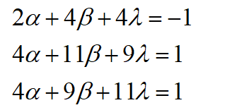
solving these equations, we get
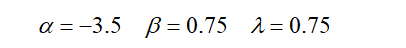
Now, we can compute weight vector of the hyperplane as below,

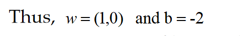
Hence, equation of hyperplane that divides data points is
X-2 = 0
Data point to be classified is (5,2) Putting this data point in above equation we get, 5-2=3 Thus the data point (5,2) belongs to +1 (Positively) class


Comments