R Exercise: Monte Carlo Simulations in R

Monte Carlo Simulations

What is Monte Carlo Simulations?

One of the main motivations to switch from spreadsheet-type tools (such as Microsoft Excel) to a program like R is for simulation modeling. R allows us to repeat the same (potentially complex and detailed) calculations with different random values over and over again.

Within the same software, we can then summarize and plot the results of these replicated calculations. Monte Carlo methods are used to perform this type of analysis they randomly sample from a set of values in order to generate and summarize a distribution of some statistic related to the sampled quantities.

Randomness

Random processes are an important aspect of simulation modeling. A random process is one that produces a different result each time it is run according to some rules. They are inextricably tied to the concept of uncertainty, you have no idea what will happen the next time the process is run.

There are two basic ways to introduce randomness in R

Random deviattes

Resampling

Random Deviates

Each person alive at the start of the year has the option of living or dying at the conclusion of the year. There are two possible endings here, and each person has an 80% probability of surviving. survive is the outcome of a binomial random process in which there were n individuals alive at the start of this year and p is the probability that any one of them would live to the next year.

In R, we can simulate a binomial random process with p=0.8 and n=100.

rbinom(n= 1, size =100,
       prob= 0.8)

## [1] 80

At this time I got 73, but we almost certainly get different number than this one.

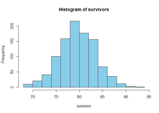
With a little tinkering, we can also plot it

survivors = rbinom(1000,
                   100, 0.8)
hist(survivors,
  col = "skyblue")

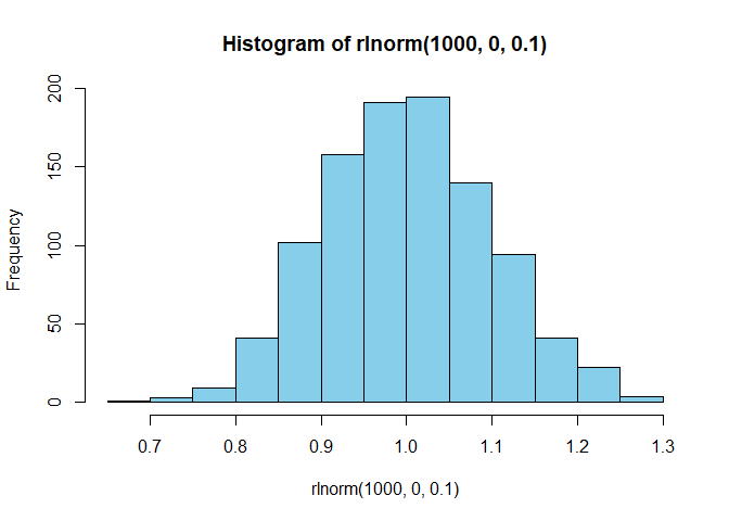
We could also used other processes like log normal

The log normal process is another random process. It creates random numbers using a log of the values that is regularly distributed, with a mean of log mean and a standard deviation of log sd.

hist(rlnorm(1000,0,0.1),col="skyblue")

Need for sampling

There are several situations in probability, and more broadly in machine learning, where an analytical solution cannot be calculated immediately. In Machine Learning, a problem of class imbalance exists. In fact, some would argue that for most practical probabilistic models, accurate inference is impossible.

The desired calculation is usually a sum of discrete distributions or an integral of continuous distributions, and thus is computationally difficult. For a variety of reasons, such as the huge number of random variables, the stochastic nature of the domain, noise in the data, a shortage of observations, and more, the calculation may be intractable.

Resampling

Using random deviates to generate fresh random numbers is excellent, but what if we already have a set of numbers to which we want to add randomness? We can utilize resampling techniques to do this. To sample size elements from the vector x in R, use the sample() function.

##Resampling of 1 to 10

sample(x = 1:10, size =5)

## [1]  4  3 10  9  2

Sample with replacement

sample(x = c("a","b","c"), size = 10, replace = T)

##  [1] "a" "a" "a" "b" "a" "b" "a" "c" "b" "b"

Sample with set probalilities

sample(x = c("live","die"),size = 10, replace = T, prob = c(0.8,0.2))

##  [1] "live" "live" "die"  "die"  "live" "live" "live" "die"  "live" "live"

Reproducing Randomness

We may want to receive the same precise random integers each time we run our script for reproducibility. To do so, we must first set the random seed, which is the starting point of our computer’s random number generator.

set.seed(1234)
rnorm(1)

## [1] -1.207066

Let’s try without random seed

rnorm(1)

## [1] 0.2774292

Each time we get different result.

Replication

To use Monte Carlo methods, we need to be able to replicate some random process many times. There are two main ways this is commonly done, either with replicate()or with for()loops.

The replicate() functions executes same expression many times and returns the output from each execution. Say we have a vector x, which represents 40 observations of an animal length(mm).

x = rnorm(30, 500,40)

We want to create the mean length sampling distribution “by hand.” We can take a random sample, determine the mean, and then repeat the process as many times as necessary.

Replication with “for” loop

A loop is a command in programming that repeats itself until it reaches a specified point. R has a few types of loops, repeat(), while(), and for(). for() loops are among the most common in simuation modeling.For each value in a vector, a for() loop performs an operation for the number of times you specify.

For loop syntax

for(var in seq){ expression(var) }

for( i in 1:5){
print(i^2)
}

## [1] 1
## [1] 4
## [1] 9
## [1] 16
## [1] 25

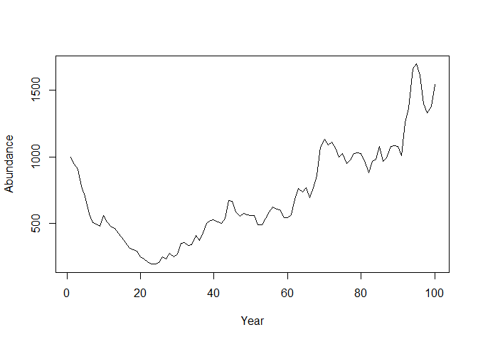
nt = 100
N= NULL
N[1] = 1000
for(t in 2:nt){
  N[t] = (N[t-1]*1.1*rlnorm(1,0,0.1))*(1-0.08)
}

Let’s plot it

plot(N, type= "l", pch = 15, xlab = "Year", ylab = "Abundance")

Summarization of simulation

After replicating a calculation many times, we will need to summarize the results.

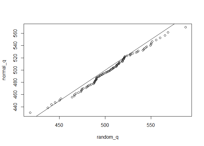
Simulating Based Learning

mu = 500
sig = 30
random = rnorm(100,mu,sig)
p = seq(0.01, 0.99, 0.01)
random_q = quantile(random,p)
normal_q = qnorm(p,mu,sig)
plot(normal_q~random_q)
abline(c(0,1))

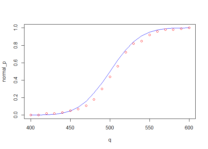
q = seq(400,600,10)
random_cdf = ecdf(random)
random_p =random_cdf(q)
normal_p = pnorm(q,mu,sig)
plot(normal_p~q, type= "l", col = "blue")
points(random_p~q,col = "red")