Previously, we wrote blogs on many machine learning algorithms as well as many other topics to help you broaden your knowledge. Please kindly visit our site and we would be glad if we got some feedback from you to improve our writing. To see some of them, you can follow the mentioned links.
Here, in this blog, we are going to discuss different types of model evaluation techniques and help which measure is suitable for your model.
Introduction
Model evaluation is a technique for determining whether a model on test data is accurate. The test data consists of information that the model has never seen before. Model selection is a method for choosing the best model once each model has been assessed against the necessary standards. Multiple measures can be used to evaluate models. However, selecting the proper evaluation metric is important and frequently depends on the issue being resolved. The evaluator can find a suitable match between the problem statement and a metric by having a thorough understanding of a variety of metrics. There are different measure of model evaluation based up on weather it is balance classification problem or imbalance classification problem.
Confusion Matrix
We must assess the performance of a classification algorithm before choosing it to tackle a problem. For calculating classification algorithm performance metrics, confusion matrices are frequently utilized. An N x N matrix called a confusion matrix is used to assess the effectiveness of a classification model, where N is the total number of target classes. In the matrix, the actual goal values are contrasted with those that the machine learning model anticipated. This gives us a comprehensive understanding of the effectiveness of our classification model and the types of mistakes it is committing. If there are only two classes then we call that classification problem as a binary classification problem however in multi-class classification problem there as more than two classes.
Model evaluation technique for binary class classification problems
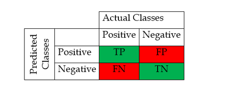
For binary classification problem there are only two classes. We used 2 by 2 matrix and there are only 4 values. Confusion matrix look like below,

True Positive: It represent the correctly classified positive classes. Here actual value is true and the machine learning model also shows a true value.
False Positive: It represent incorrectly classified positive classes. Here actual value is false but model shows the true value. It is also called type I error.
True Negative: It represent correctly classified negative classes. Here actual and predicated both values are negative.
False Negative: It represent incorrectly classified negative classes. Here actual value is true but model predict false value. It is also called type II error.
Accuracy, recall, precision, and F1-score are four often used performance metrics for assessing classification algorithms.
Accuracy: It is indicated as follows and represents the model’s proportion of accurate predictions.
Accuracy = (TP + TN)/(TP + TN + FP + FN)
Precision: It is percentage of predicted positives that are actually positive and is given by,
Precision = TP/(TP + FP)
Recall: It is the percentage of actual positives that are correctly classified by the model and is given as below,
Recall = TP/(TP + FN)
F1-Score: It is the harmonic mean of recall and precision. It becomes high only when both precision and recall are high. This score is given by,
F1-scoare = (2 * Recall * Precision)/(Recall + Precision)
On unbalanced problems, accuracy should not be used. Then, by simply identifying all observations as belonging to the majority class, it is simple to obtain a high accuracy score. The F1-score is a popular metric for imbalanced classification.
Sensitivity-Specificity Metrics: Sensitivity is a measure of how accurately the positive class was predicted and corresponds to the genuine positive rate.
Sensitivity = Recall = TP/(TP + FN)
The complement of sensitivity, often known as the genuine negative rate, is called specificity. It quantifies how well the negative class was anticipated.
specificity = TN/(FP + TN)
ROC Curve: The true positive rate versus false positive rate is plotted on the ROC curve. Receiver operating characteristics are referred to as ROCs. True positive rate is also called and recall and is give by,
True Positive rate/Recall/Sensitivity = TP/(TP + FN)
False Positive rate = FP/(FP + TN) = 1- specificity
The performance of the model is improved if the area under the ROC curve is bigger. If the curve is close to the 50% diagonal line, the output variable may be predicted arbitrarily by the model.
Log Loss: A particularly efficient classification metric is log loss, which is equal to -1*log (likelihood function), where likelihood function denotes the model’s estimation of the likelihood of the observed set of events. Since the likelihood function returns relatively small values, changing the numbers to log and adding the negative to them improves their interpretation, making a smaller loss score suggest a better model.
Regression Matrix
In contrast to classification models, which have discrete output variables, regression models offer a continuous output variable. As a result, the metrics for evaluating the regression models are created appropriately. Some of the widely used regression metrics are: MSE, RMSE, RMSLE, MAE, R2.
Mean Squared Error (MSE): The MSE is a straightforward measure that computes the error—the difference between the actual value and the predicted value—squares it, and then outputs the average of all the errors.

Where y is actual value and ŷ is predicted value.
MSE is very sensitive to outliers and will show a very high error value even if a few outliers are present in the otherwise well-fitted model predictions
Root Mean Squared Error (RMSE): The benefit of RMSE, which is the source of MSE, is that it lowers the magnitude of the errors so that they are more interpretable and closer to the true values.
Mean Absolute Error or MAE: MAE is the mean of the absolute error values (actuals – predictions)

MAE is the best option if one wants to partially ignore the outlier values because the elimination of the square terms greatly lowers the outliers’ penalty.
Root Mean Squared Log Error (RMSLE) The equation for RMSLE is the same as for RMSE, with the addition of a log function along with the actual and forecasted values.

This minimizes the greater error rates using the log function, which lessens the impact of the outliers.
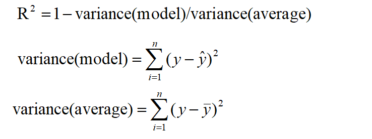
R-squared (R^2): R-Square calculates the percentage of the dependent variable’s variance that is explained by the independent variable.

R^2 squared basically determines whether a regression line is superior to a mean line. A higher R squared value denotes a more favorable match. R^2 squared is hence sometimes known as the coefficient of determination or occasionally as the goodness of fit. R^2 scores might be between 0 and 1. The R^2 value should be as near to 1 as possible. The model is not doing any better than a random model if R^2 is equal to 0.
Adjusted R^2: The R^2 score’s drawback is that it never decreases as new characteristics are added to the data since it expects that the variance of the data would increase as more data are added. The issue is that sometimes R^2 starts to increase incorrectly when we add an unrelated feature to the dataset. In order to manage this scenario, Adjusted R Squared was created.

Where, n is number of observations, k is number of independent variables, and Ra^2 is adjusted R^2
-
Now as K increases by adding some irrelevant features so the denominator will decrease, n-1 will remain constant. R^2 score will remain constant or will increase slightly so the complete term will increase and when we subtract this from one then the resultant score will decrease.
-
And if we add a relevant feature then the R2 score will increase and 1-R2 will decrease heavily and the denominator will also decrease so the complete term decreases, and on subtracting from one the score increases.
Clustering Matrix
Because clustering algorithms identify groups of data points, distance-based metrics work well in this situation. The Dunn Index, Silhouette Coefficient, Elbow technique, and others are some of the most popular clustering metrics.
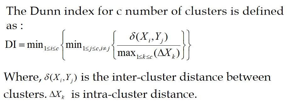
Dunn Index: A statistic for assessing clustering algorithms is the Dunn index (DI). The purpose of this Dunn index is to find groups of clusters that are well separated, compact, and have little variation between their individual members. It is determined as the smallest intra-cluster distance divided by the smallest inter-cluster distance (i.e., the distance between any two cluster centroids).

The clustering is more favorable the higher the Dunn index value. The optimal number of clusters, k, is determined by maximizing the Dunn index. It also has several shortcomings. The computing cost rises along with the data’s size and number of clusters.
Silhouette Coefficient: Another statistic used to assess the effectiveness of a clustering method is the silhouette coefficient, often known as the silhouette score. Its value is between -1 and 1. Silhouette Score = (b-a)/max(a,b)
where, a = average intra-cluster distance, b = average nearest inter-cluster distance.
The ideal value is 1, whereas the undesirable value is -1. Values close to 0 signify clusters that overlap. Negative results typically signify that a sample was placed in the incorrect cluster because another cluster would have better fit the sample.
Elbow Method: Plotting the number of clusters on the x-axis against the proportion of variance explained on the y-axis yields the number of clusters in a dataset using the elbow technique. The elbow in the x-axis is thought to suggest the ideal number of clusters because it marks where the curve abruptly bends.


Comments