Kmeans Clustering in Python from Scratch

Introduction

K mean clustering is very simple type of unsupervised learning. Which is used to solve clustering problem. Using this algorithm we can easily classify given data point in given clusters. To do so we should first find number of cluster. In k mean cluster it is highly except that inter-cluster cluster is low and intra cluster distance is high. We should give concern while using k mean because different location give different result so, better choice us to place them as much as possible far away from each other.

Algorithm

Let $P = {p_1,p_2,p_3,…,p_n}$ be the set of data points and $C = {c_1,c_2,c_3,…,c_n}$ be the set of centers.

Step 1: Initially randomly select appropriate numbers of “c” cluster center.

Step 2: Calculate distance between each data point $P = {p_1,p_2,p_3,…,p_n}$ and cluster center ‘c’.

Step 3:Kept data points to the cluster center whose distance from the cluster center is minimum of all the cluster centers.

Here we calculate the distance using euclidean distance. Mathematically,\(= \sum_{i=1}^n (x_i^2-y_i^2)\)

Step 4: Now, recalculate the new cluster center using \(\frac{1}{c}\sum_{i=1}^c x_i\) where $c_i$ represent the number of data point in $i^th$ clusters.

Step 5: Again calculate the distance between new cluster centers and each data points.

Step 6: If number of data points in a cluster are updated then repeat step3 otherwise terminate.

Example

Divide the data points ${(1,1),(2,1),(4,3),(5,4)}$ using k-mean clustering into 2 clusters.

Solution

Let $p_1 = (1,1), P_2 =(2,1), P_3 =(4,3), p_4 = (5,4) $

Step1

Let $c_1=(1,1)$ and $c_2=(2,1)$ are two initial cluster centers.

Iteration I Now, calculate distance between clusters centers and each data points.

$d(c_1,p_1)=0$

$ d(c_2,p_1) = \sqrt{(2-1)^2+(1-1)^2} = 1$

$ d(c_1,p_2) = \sqrt{(2-1)^2+(1-1)^2} = 1$

$d(c_2,p_2)=\sqrt{(2-2)^2+(1-1)^2} = 0$

$ d(c_1,p_3) = \sqrt{(4-1)^2+(3-1)^2} = 3.6$

$ d(c_2,p_3) = \sqrt{(4-2)^2+(3-1)^2} = 2.83$

$ d(c_1,p_4) = \sqrt{(5-1)^2+(4-1)^2} = 5$

$ d(c_2,p_4) = \sqrt{(5-2)^2+(4-1)^2} = 4.24$

Thus, we found following clusters

• Cluster 1 = {$p_1$}

• Cluster 2 = {$p_2, p_3, p_4$}

Now, new cluster centers are:

$c_1 = (1,1)$ and $c_2 = (\frac{(2+4+5)}{3}, \frac{(1+3+4)}{3}) = (\frac{11}{3}, \frac{8}{3})$

Iteration2

Calculate the distance between new cluster centers and each data points.

$d(c_1, P_1) =0$

$ d(c_2,p_1) = \sqrt{(\frac{11}{3}-1)^2+(\frac{8}{3}-1)^2} = 3.14$

$ d(c_1,p_2) = \sqrt{(2-1)^2+(1-1)^2} = 1$

$ d(c_2,p_2) = \sqrt{(\frac{11}{3}-2)^2+(\frac{8}{3}-1)^2} = 2.35$

$ d(c_1,p_3) = \sqrt{(4-1)^2+(3-1)^2}=3.6 $

$ d(c_2,p_3) = \sqrt{(\frac{11}{3}-4)^2+(\frac{8}{3}-3)^2} = 0.46$

$ d(c_1,p_4) = \sqrt{(5-1)^2+(4-1)^2} = 5$

$ d(c_2,p_4) = \sqrt{(\frac{11}{3}-5)^2+(\frac{8}{3}-4)^2} = 1.88$

So, cluster form after second iteration is,

• Cluster 1 = {$p_1, p_2$}

• Cluster 2 = {$P_3,p_4$}

Again new centers are

$ c_1$ = $\frac{(1+2)}{2}$,$\frac{(1+1)}{2} $ and $ c_2$ = $\frac{(2+4+5)}{3}$,$\frac{(1+3+4)}{3}$ = $(\frac{11}{3},\frac{8}{3})$

Repeat this process till no re-assignment of points to groups.

Applications

• Customer segmentation
• Image segmentation
• Document segmentation

Advantages

• Fast, robust and easier to understand.
• Gives best result when data set are distinct or well separated from each other.

Disadvantages

• The learning algorithm requires apriori specification of the number of cluster centers.
• Randomly choosing of the cluster center cannot lead us to the fruitful result.
• Applicable only when mean is defined i.e. fails for categorical data.
• Algorithm fails for non-linear data set.

Coding Part

Imports

import numpy as np
import matplotlib.pyplot as plt

plt.style.use("seaborn-whitegrid")

Basic Example

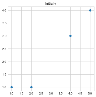
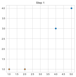
Lets take an example of above data points where we had 4 points and we will try to make 2 clusters for those data.

1. Initially, we will plot our data points by passing x and y coordinates of all points.
2. Take point 1st and 2nd as initial center points or center of two clusters.

points = np.array([(1,1),(2,1),(4,3),(5,4)])

print(points)

plt.figure(figsize=(5,5))
plt.scatter(x=points[:,0],y = points[:,1])
plt.title("Initially")
plt.show()

k = 2
c1 = points[0]
c2 = points[1]

plt.figure(figsize=(5,5))
plt.scatter(x=points[:,0],y = points[:,1])
plt.scatter([c1[0],c2[0]],[c1[1],c2[1]],marker="*")
plt.title("Step 1")
plt.show()

[[1 1]
 [2 1]
 [4 3]
 [5 4]]

1. Make a function distance to calculate 2d distance between point and a center of cluster.
2. Now, loop through number of steps that we want to perform
   4.i. Initialize an empty clusters because we will swap points in between in each steps.
   4.ii. Loop through each data points 4.ii.a. If a distance between point and center of cluster 1 is smaller than that with cluster 2 then we will assume that this point lies in cluster 1. Else it will lie in cluster 2. 4.iii. Recalculate centers from each clusters. 4.iv. Plot cluster center and points.

def distance(p1, p2):
    return np.sqrt((p1[0]-p2[0])**2 + (p1[1]-p2[1])**2)
print(distance((1,2),(2,3)))

c1 = points[0]
c2 = points[1]

    
for i in range(5):
    clusters = {i: [] for i in range(k)}
    for point in points:
        d1 = distance(point,c1)
        d2 = distance(point,c2)
        #print(point,d1,d2,c1,c2)
        if d1 < d2:
            clusters[0].append(point)
        else:
            clusters[1].append(point)
    print(f"Step {i}. {clusters}")
    
    clusters = {k: np.array(v) for k,v in clusters.items()}
    
    c1= np.array(clusters[0]).mean(axis=0)
    c2 = np.array(clusters[1]).mean(axis=0)
    
    plt.title(f"Step: {i+1}")
    plt.scatter(clusters[0][:,0], clusters[0][:,1], marker="+")
    plt.scatter(clusters[1][:,0], clusters[1][:,1], marker="*")
    plt.show()
            
        
        

1.4142135623730951
Step 0. {0: [array([1, 1])], 1: [array([2, 1]), array([4, 3]), array([5, 4])]}

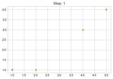
Step 1. {0: [array([1, 1]), array([2, 1])], 1: [array([4, 3]), array([5, 4])]}

Step 2. {0: [array([1, 1]), array([2, 1])], 1: [array([4, 3]), array([5, 4])]}

Step 3. {0: [array([1, 1]), array([2, 1])], 1: [array([4, 3]), array([5, 4])]}

Step 4. {0: [array([1, 1]), array([2, 1])], 1: [array([4, 3]), array([5, 4])]}

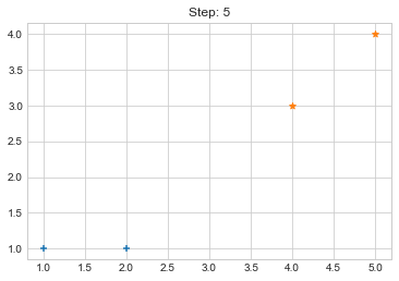
Now looking over the output of our code, it seems that it worked pretty well but what if our cluster size is variable and data also varies? So to make our code little bit more awesome, we will do few more tasks.

KMean Class

Some of reasons that we are using a class are:

1. To make our code dynamic.
2. To wrap useful methods.
3. To make it reusable without changing a structure.

Lets take it into action.

Initializing

1. Initialize class by giving data, number of clusters we want, number of steps to loop.
2. Make attributes of those values.
3. Take k number of centers serially for the sake of simplicity.
4. Prepare random color for each cluster.

class KMean:
    def __init__(self,data,k,steps):
        self.data= data
        self.k = k
        self.steps = steps
        self.centers = np.array([self.data[i] for i in range(self.k)])
        self.colors = np.array(np.random.randint(0, 255, size =(self.k, 4)))/255
        self.colors[:,3]=1

distance method

Just to find distance.

    def distance(self,p1,p2):
        return np.sqrt((p1[0]-p2[0])**2 + (p1[1]-p2[1])**2)

initialize method

Just to view initial plots.

    def initialize(self):
        """
            Initialize the Clusters.
        """
        self.clusters = {i: [] for i in range(self.k)}
        plt.scatter(self.centers[:, 0], self.centers[:, 1], s=200, color=self.colors)
        plt.scatter(self.data[:, 0], self.data[:,1],marker="*", s=100)
        plt.title("Initialize")
        plt.show()

fit method

This method will implement everything we did in above simple example.

    def fit(self):
        for step in range(self.steps):
            self.clusters = {i: [] for i in range(self.k)}
            
            for point in self.data:
                d= np.array([self.distance(point,c) for c in self.centers])
                c = np.argmin(d)
                self.clusters[c].append(point)
                
            self.clusters= {i:np.array(v) for i,v in self.clusters.items()}
            self.centers = np.array([self.clusters[i].mean(axis=0) for i in range(self.k)])
            self.visualize(step= step)

visualize method

To visualize our data points and cluster centers.

    def visualize(self,step):
        plt.title(f"Step : {step}")
        [plt.scatter(self.clusters[i][:, 0], self.clusters[i][:, 1], marker="*", s=100,
                    color = self.colors[i]) for i in range(self.k)]
        plt.scatter(self.centers[:, 0], self.centers[:, 1], s=200, color=self.colors)
        plt.show()

Now lets see it all in combined form.

All Codes

class KMean:
    def __init__(self,data,k,steps):
        self.data= data
        self.k = k
        self.steps = steps
        self.centers = np.array([self.data[i] for i in range(self.k)])
        self.colors = np.array(np.random.randint(0, 255, size =(self.k, 4)))/255
        self.colors[:,3]=1
        
    def distance(self,p1,p2):
        return np.sqrt((p1[0]-p2[0])**2 + (p1[1]-p2[1])**2)
        
    def initialize(self):
        """
            Initialize the Clusters.
        """
        self.clusters = {i: [] for i in range(self.k)}
        plt.scatter(self.centers[:, 0], self.centers[:, 1], s=200, color=self.colors)
        plt.scatter(self.data[:, 0], self.data[:,1],marker="*", s=100)
        plt.title("Initialize")
        plt.show()
        
    def fit(self):
        for step in range(self.steps):
            self.clusters = {i: [] for i in range(self.k)}
            
            for point in self.data:
                d= np.array([self.distance(point,c) for c in self.centers])
                c = np.argmin(d)
                self.clusters[c].append(point)
                
            self.clusters= {i:np.array(v) for i,v in self.clusters.items()}
            self.centers = np.array([self.clusters[i].mean(axis=0) for i in range(self.k)])
            self.visualize(step= step)
            
    def visualize(self,step):
        plt.title(f"Step : {step}")
        [plt.scatter(self.clusters[i][:, 0], self.clusters[i][:, 1], marker="*", s=100,
                    color = self.colors[i]) for i in range(self.k)]
        plt.scatter(self.centers[:, 0], self.centers[:, 1], s=200, color=self.colors)
        plt.show()
    
    

Test it!

kmean = KMean(points, 2, 5)
kmean.initialize()
kmean.fit()

kmean.centers

array([[1.5, 1. ],
       [4.5, 3.5]])

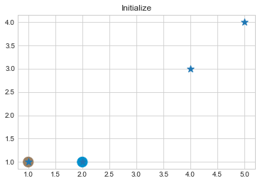
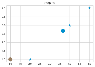
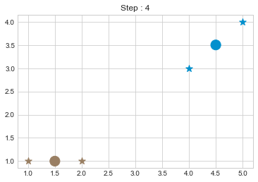
As we can see in above outputs, the center of clusters are larger than points and in early steps, the points has been changed from one cluster to another.

With more data

Lets make an random data with 100 points and test on it.

x = np.arange(0, 100)
y = np.random.randint(0, 100, 100)

plt.scatter(x,y)
plt.show()

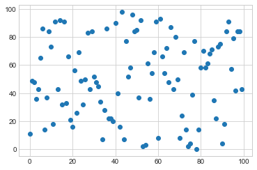
Now lets choose 5 clusters and see how it works over a time of 10 steps.

data = np.array([(x[i], y[i]) for i in range(100)])

km1 = KMean(data,k=5,steps=10)
km1.initialize()
km1.fit()

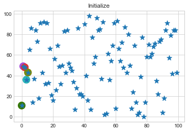
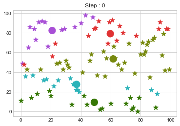
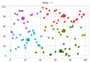
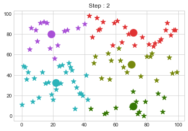
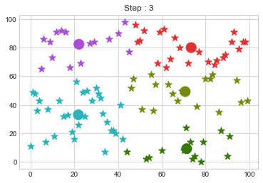
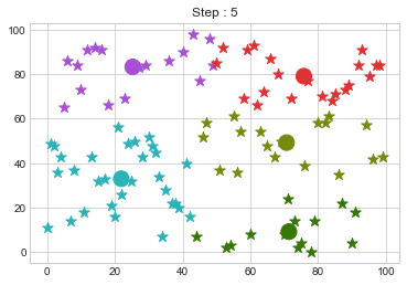
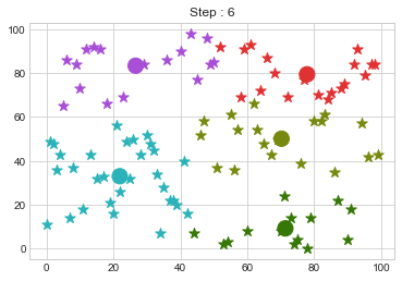
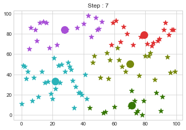
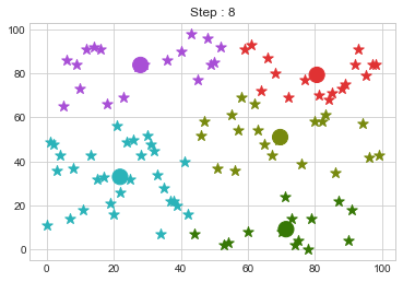
Lets focus on the step 0 to 3, can you see the points moving from one cluster to another? But as the steps increased, our data clustering became stable.

Outliers

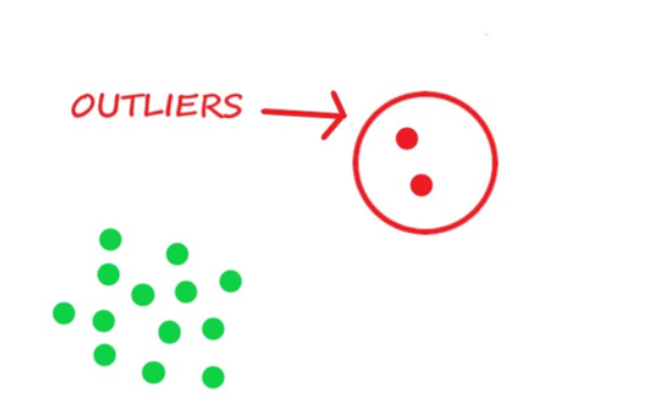
One of major disadvantage of KMeans Clustering is Outliers. It is very sensible to outliers and lets see how and what will be the solution of it? Lets use data from above step and modify 3 points.

data = np.array([(x[i], y[i]) for i in range(100)])
data[0] = [120, 100]
data[50] = [-30, 120]
data[99] = [100, -50]

km2 = KMean(data,k=5,steps=10)
km2.initialize()
km2.fit()

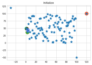
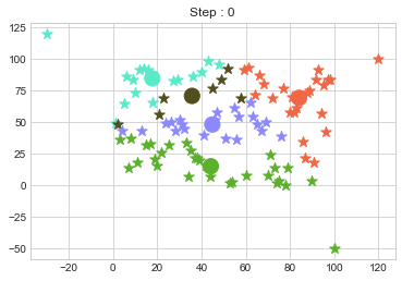
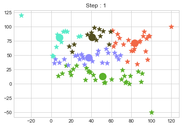
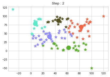
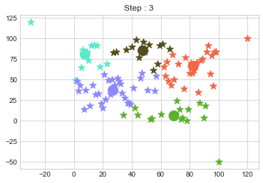
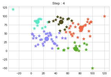
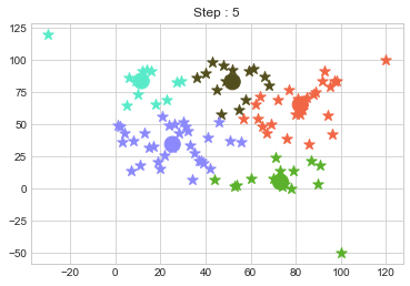
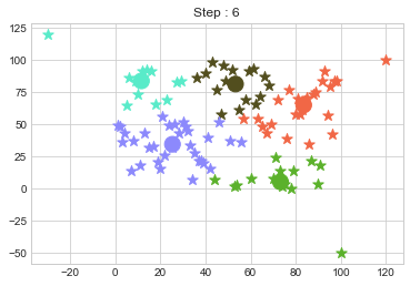
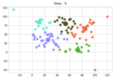
In above step, we have changed only 3 points and the affect of it is huge. But lets see how huge it is by comparing its center points.

km1.centers, km2.centers

(array([[71.35714286,  9.28571429],
        [28.        , 83.78947368],
        [80.52941176, 79.29411765],
        [21.93333333, 33.03333333],
        [69.6       , 51.05      ]]),
 array([[84.66666667, 65.41666667],
        [11.58333333, 83.66666667],
        [53.52941176, 79.64705882],
        [73.26666667,  5.33333333],
        [25.34375   , 34.53125   ]]))

Comparing the length of clusters.

[len(c) for c in km1.clusters.values()], [len(c) for c in km2.clusters.values()]

([14, 19, 17, 30, 20], [24, 12, 17, 15, 32])

Which clearly shows that most of the cluster’s points has been changed due to outliers. Now comes the part of solution. There is not a solution of outliers in KMeans Clustering but a variant of it, KMedoids is used in those case. We will share it in next blog. :)