
Data Analysis Using Pipe Operator in R
What is pipe oprator?
Pipe operators are strong tools for expressing a series of numerous operations in a clear and concise manner. The pipe is a part of the magrittr package. Pipe allows us to write code in a more readable and understandable manner. Lets see how.
Why to use Pipe?
Because R is a functional and complicated programming language which frequently necessitates a lot of parenthesis, which means we have to nest those parenthesis together for statistical computing. R codes are difficult to read and comprehend as a result of this. This is when the suitation pipe comes in handy. Pipe operators are divided into three categories. They are,
- Compund Operator
- Tee Operator
- S Operator
%< >% Compound Operator
Compound operator updates the values for same variable.
x <- rnorm(100)
x %<>% abs %>% sort
x
##   [1] 0.009983937 0.016608923 0.023887211 0.028489290 0.058244965 0.077193140
##   [7] 0.112791553 0.120680475 0.142512597 0.146191765 0.147149809 0.165798798
##  [13] 0.169114223 0.178767244 0.186996059 0.215662105 0.225165303 0.225711892
##  [19] 0.234813083 0.255162793 0.257619673 0.263657947 0.274256886 0.278533752
##  [25] 0.294561592 0.301091692 0.303962890 0.341956524 0.344785272 0.356188353
##  [31] 0.364966970 0.386465486 0.392640172 0.397031027 0.399785232 0.401835250
##  [37] 0.454831319 0.462229304 0.480710234 0.483437251 0.483892691 0.486781500
##  [43] 0.495098266 0.500368634 0.552609131 0.557855069 0.562689263 0.569710993
##  [49] 0.570507316 0.579221386 0.645926049 0.647673949 0.651625795 0.669647688
##  [55] 0.685098831 0.691043660 0.695729376 0.718395762 0.735014583 0.806662050
##  [61] 0.829931993 0.864247899 0.872475691 0.885884373 0.894854852 0.905258561
##  [67] 0.913041727 0.956071568 1.034663289 1.037072257 1.046854227 1.123876928
##  [73] 1.155893261 1.160593930 1.170788411 1.182924108 1.202387282 1.273220874
##  [79] 1.273903761 1.306092878 1.322683135 1.338790649 1.347844508 1.351232284
##  [85] 1.361332556 1.389807581 1.392778554 1.421035715 1.444100750 1.480067832
##  [91] 1.603077777 1.618609928 1.633015485 1.682547525 1.703995370 1.709338446
##  [97] 1.750947764 1.817871496 2.289798927 2.358908977
Here at first, %<>% finds the absolute values of x and and then it sorts in increasing order.
%>% tee Operator
Normally, the code ends after plot command but the tee pipe operator
allows it to continue for the next argument.
set.seed(123)
rnorm(200) %>%
matrix(ncol = 2) %T>%
plot %>%
colSums
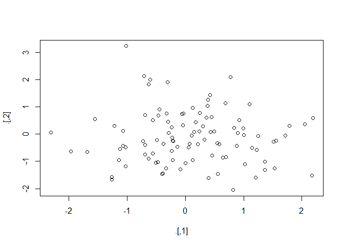
## [1] 9.040591 -10.754680
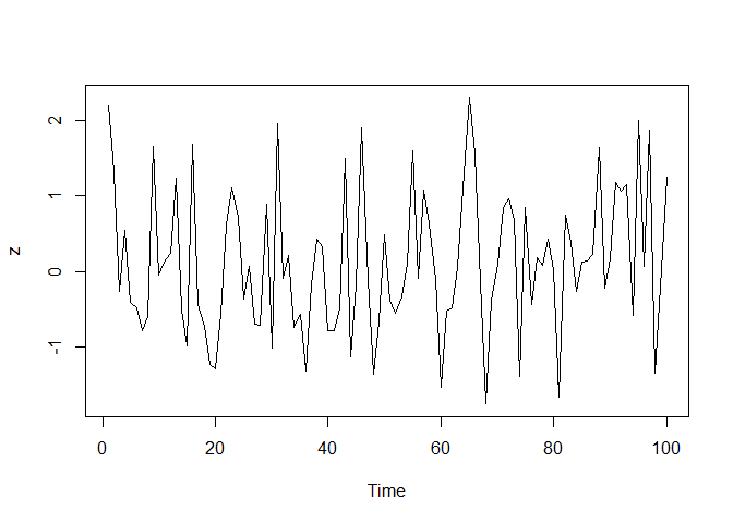
%$%
This operator is useful when we want to pipe a dataframe which may contains many columns in to a function that is applied to some of the columns.
data.frame(z = rnorm(100)) %$%
ts.plot(z)
Let’s do some Data Analysis in iris data with Pipe Operator
First, let’s us check what attributes iris data contains.
head(iris)
##   Sepal.Length Sepal.Width Petal.Length Petal.Width Species
## 1          5.1         3.5          1.4         0.2  setosa
## 2          4.9         3.0          1.4         0.2  setosa
## 3          4.7         3.2          1.3         0.2  setosa
## 4          4.6         3.1          1.5         0.2  setosa
## 5          5.0         3.6          1.4         0.2  setosa
## 6          5.4         3.9          1.7         0.4  setosa
Here, iris data have four columns they are
Sepal.Length,Sepal.Width, Petal.Length ,Petal.Width Species.
library(dplyr)
##
## Attaching package: 'dplyr'

## The following objects are masked from 'package:stats':
##
##     filter, lag

## The following objects are masked from 'package:base':
##
##     intersect, setdiff, setequal, union
iris %>%
  select(contains('Sepal')) %>%
  mutate(Sepal.Area=Sepal.Length * Sepal.Width)
##     Sepal.Length Sepal.Width Sepal.Area
## 1            5.1         3.5      17.85
## 2            4.9         3.0      14.70
## 3            4.7         3.2      15.04
## 4            4.6         3.1      14.26
## 5            5.0         3.6      18.00
## 6            5.4         3.9      21.06
## 7            4.6         3.4      15.64
## 8            5.0         3.4      17.00
## 9            4.4         2.9      12.76
## 10           4.9         3.1      15.19
## 11           5.4         3.7      19.98
## 12           4.8         3.4      16.32
## 13           4.8         3.0      14.40
## 14           4.3         3.0      12.90
## 15           5.8         4.0      23.20
## 16           5.7         4.4      25.08
## 17           5.4         3.9      21.06
## 18           5.1         3.5      17.85
## 19           5.7         3.8      21.66
## 20           5.1         3.8      19.38
(Only first 20 rows are shown.)
contains function only selects those columns which contains sepal
word. Here we have also imported dplyr using library(dplyr). dplyr package is mainly used
for data cleaning purpose. It contaims five buitin function they are:
- select
- filter
- arrange
- mutate
These five functions can do majority of data manipulatlation for data analysis task.
In above code mutate function added new column (Sepal.Area) in the
data frame.
iris %>%
  select(starts_with('Sepal')) %>%
  filter(Sepal.Length >= 5.0) %>%
  arrange(Sepal.Length)
##     Sepal.Length Sepal.Width
## 1            5.0         3.6
## 2            5.0         3.4
## 3            5.0         3.0
## 4            5.0         3.4
## 5            5.0         3.2
## 6            5.0         3.5
## 7            5.0         3.5
## 8            5.0         3.3
## 9            5.0         2.0
## 10           5.0         2.3
## 11           5.1         3.5
## 12           5.1         3.5
## 13           5.1         3.8
## 14           5.1         3.7
## 15           5.1         3.3
## 16           5.1         3.4
## 17           5.1         3.8
## 18           5.1         3.8
## 19           5.1         2.5
## 20           5.2         3.5
(only first 20 rows are shown.)
By using above we can select only those columns which has
Sepal as prefix and want to filter those values which have values
greater than Sepal.Length >= 5.0 and finally we did arrange in
ascending order. If we need to sort in descending order we simply need to type
desc inside arrange function as like below.
iris %>%
  select(starts_with('Sepal')) %>%
  filter(Sepal.Length >= 5.0) %>%
  arrange(desc(Sepal.Length))
##     Sepal.Length Sepal.Width
## 1            7.9         3.8
## 2            7.7         3.8
## 3            7.7         2.6
## 4            7.7         2.8
## 5            7.7         3.0
## 6            7.6         3.0
## 7            7.4         2.8
## 8            7.3         2.9
## 9            7.2         3.6
## 10           7.2         3.2
## 11           7.2         3.0
## 12           7.1         3.0
## 13           7.0         3.2
## 14           6.9         3.1
## 15           6.9         3.2
## 16           6.9         3.1
## 17           6.9         3.1
## 18           6.8         2.8
## 19           6.8         3.0
## 20           6.8         3.2
(Only 20 rows are shown.)
Let’s try one different step
Let’s observe what will come in result if we use end_with in place
of starts_with.
iris %>%
  select(ends_with('Length')) %>%
  rowwise() %>%
  mutate(Length.Diff = Sepal.Length- Petal.Length)
## # A tibble: 150 x 3
## # Rowwise:
##    Sepal.Length Petal.Length Length.Diff
##           <dbl>        <dbl>       <dbl>
##  1          5.1          1.4         3.7
##  2          4.9          1.4         3.5
##  3          4.7          1.3         3.4
##  4          4.6          1.5         3.1
##  5          5            1.4         3.6
##  6          5.4          1.7         3.7
##  7          4.6          1.4         3.2
##  8          5            1.5         3.5
##  9          4.4          1.4         3
## 10          4.9          1.5         3.4
## # ... with 140 more rows
I hope we have observed what new came here. Here, we got prefix as Length. It means we got only those columns which has length as it’s prefix. Also by using mutate function we created new column Length.Diff.
Use transmute function
iris %>%
  select(contains('Sepal'), Species) %>%
  transmute(Sepal.Area= Sepal.Length * Sepal.Width)
##     Sepal.Area
## 1        17.85
## 2        14.70
## 3        15.04
## 4        14.26
## 5        18.00
## 6        21.06
## 7        15.64
## 8        17.00
## 9        12.76
## 10       15.19
## 11       19.98
## 12       16.32
## 13       14.40
## 14       12.90
## 15       23.20
## 16       25.08
## 17       21.06
## 18       17.85
## 19       21.66
## 20       19.38
(Only 20 rows are shown.)
Here, transmute funtion only show new columns it hide Sepal.Length
and Sepal.Width columns.
What differences can we observe when we use pipe operator and genral R function?
Let us finalize it from code,
Using R general function
Assign value of x with given column vector.
x <- c(0.109, 0.359, 0.63, 0.996, 0.515, 0.142, 0.017, 0.829, 0.907)
Here, we want to compute the following within single line of code,
- Compute the logarithm of
x, - return suitable lagged and iterated difference
- compute the exponential function and round the result
round(exp(diff(log(x))), 1)
## [1] 3.3 1.8 1.6 0.5 0.3 0.1 48.8 1.1
Let’s to some code using pipe operators.
x %>%log() %>%
  diff() %>%
  exp()%>%
  round(1)
## [1] 3.3 1.8 1.6 0.5 0.3 0.1 48.8 1.1
In above situation, pipe comes handy because we did not need to nest with lots of parenthesis. Finally we got the same result.
However, there are lots of advantages of pipe operator but there are some limitations as well while using pipe operator. Following are the some of the limitations of pipe operators.
- Our pipes are longer than (say) ten steps
- We have multiple inputs or outputs
- We are starting to think about a directed graph with a complex dependency structure
- We’re doing internal package development


Comments