
Check the data mtcars with head and save a new data as mtcars.subset after dropping two non-numeric (binary) variables for PCA analysis
data <- mtcars
head(data)
##                    mpg cyl disp  hp drat    wt  qsec vs am gear carb
## Mazda RX4         21.0   6  160 110 3.90 2.620 16.46  0  1    4    4
## Mazda RX4 Wag     21.0   6  160 110 3.90 2.875 17.02  0  1    4    4
## Datsun 710        22.8   4  108  93 3.85 2.320 18.61  1  1    4    1
## Hornet 4 Drive    21.4   6  258 110 3.08 3.215 19.44  1  0    3    1
## Hornet Sportabout 18.7   8  360 175 3.15 3.440 17.02  0  0    3    2
## Valiant           18.1   6  225 105 2.76 3.460 20.22  1  0    3    1
str(data)
## 'data.frame':    32 obs. of  11 variables:
##  $ mpg : num  21 21 22.8 21.4 18.7 18.1 14.3 24.4 22.8 19.2 ...
##  $ cyl : num  6 6 4 6 8 6 8 4 4 6 ...
##  $ disp: num  160 160 108 258 360 ...
##  $ hp  : num  110 110 93 110 175 105 245 62 95 123 ...
##  $ drat: num  3.9 3.9 3.85 3.08 3.15 2.76 3.21 3.69 3.92 3.92 ...
##  $ wt  : num  2.62 2.88 2.32 3.21 3.44 ...
##  $ qsec: num  16.5 17 18.6 19.4 17 ...
##  $ vs  : num  0 0 1 1 0 1 0 1 1 1 ...
##  $ am  : num  1 1 1 0 0 0 0 0 0 0 ...
##  $ gear: num  4 4 4 3 3 3 3 4 4 4 ...
##  $ carb: num  4 4 1 1 2 1 4 2 2 4 ...
In our data vs and am are binary variable so I drop them here.
library(dplyr)
mtcars.subset <- data[,-c(8,9)]
Fit PCA in the data by mtcars.pca matcars.subset with cor = TRUE and scores = TRUE
mtcars.pca<-prcomp(mtcars.subset, cor = TRUE, scores = TRUE)
## Warning: In prcomp.default(mtcars.subset, cor = TRUE, scores = TRUE) :
##  extra arguments 'cor', 'scores' will be disregarded
Get summary of mtcars.pca
summary(mtcars.pca)
## Importance of components:
##                            PC1      PC2     PC3     PC4     PC5     PC6    PC7
## Standard deviation     136.532 38.14735 3.06642 1.27492 0.90474 0.64734 0.3054
## Proportion of Variance   0.927  0.07237 0.00047 0.00008 0.00004 0.00002 0.0000
## Cumulative Proportion    0.927  0.99938 0.99985 0.99993 0.99997 0.99999 1.0000
##                           PC8    PC9
## Standard deviation     0.2859 0.2159
## Proportion of Variance 0.0000 0.0000
## Cumulative Proportion  1.0000 1.0000
From above summary we see when standard deviation is greater propertion of variance is high similarly when standard deviation is low propertion of variation is also low.
Get eigenvalue of the components using standard deviation of mtcars.pca and chose the number of components based on Kaiser’s criteria
mtcars.pca$sdev ^2
## [1] 1.864106e+04 1.455220e+03 9.402948e+00 1.625431e+00 8.185525e-01
## [6] 4.190430e-01 9.327903e-02 8.175127e-02 4.660443e-02
Get scree plot and chose the number of components best on “first bend” of this plot
#Calculating total variance explained by each principal component
var_explained<-mtcars.pca$sdev^2/sum(mtcars.pca$sdev^2)
##Creating scree plot
library(ggplot2)
qplot(c(1:9), var_explained) + geom_line() + xlab("Principal Component") + ylab("Variance explained") + ggtitle("Scree Plot")
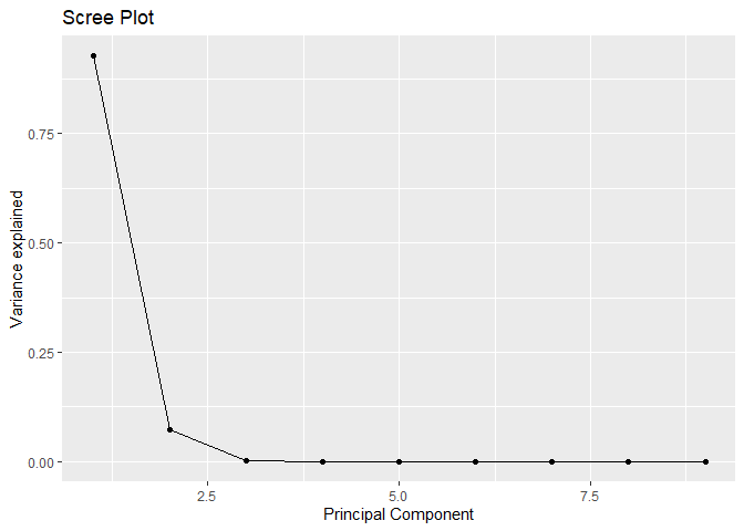
How many components must be retained based on Kaiser’s rule and/or scree plot?
Kisher’s rule suggaest us to use 2 components and Scree plot suggest us to retain 4 components for the problem.
Fit the final PCA model based on the retained components
library(psych)
## Warning: package 'psych' was built under R version 4.1.2
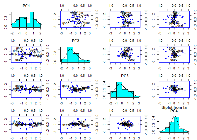
mtcars.pca<- psych::principal(mtcars.subset, nfactors = 4, rotate = "none")
mtcars.pca
## Principal Components Analysis
## Call: psych::principal(r = mtcars.subset, nfactors = 4, rotate = "none")
## Standardized loadings (pattern matrix) based upon correlation matrix
##        PC1   PC2   PC3   PC4   h2     u2 com
## mpg  -0.93  0.04 -0.16  0.00 0.90 0.0995 1.1
## cyl   0.96  0.02 -0.18  0.02 0.95 0.0504 1.1
## disp  0.94 -0.13 -0.06  0.17 0.94 0.0569 1.1
## hp    0.87  0.39 -0.01  0.04 0.91 0.0854 1.4
## drat -0.74  0.49  0.11  0.44 0.99 0.0062 2.5
## wt    0.89 -0.25  0.32  0.10 0.96 0.0360 1.5
## qsec -0.53 -0.70  0.45 -0.02 0.97 0.0283 2.6
## gear -0.50  0.79  0.15 -0.15 0.92 0.0775 1.8
## carb  0.58  0.70  0.33 -0.11 0.95 0.0525 2.5
##
##                        PC1  PC2  PC3  PC4
## SS loadings           5.66 2.08 0.50 0.27
## Proportion Var        0.63 0.23 0.06 0.03
## Cumulative Var        0.63 0.86 0.92 0.95
## Proportion Explained  0.66 0.24 0.06 0.03
## Cumulative Proportion 0.66 0.91 0.97 1.00
##
## Mean item complexity =  1.7
## Test of the hypothesis that 4 components are sufficient.
##
## The root mean square of the residuals (RMSR) is  0.02
##  with the empirical chi square  0.96  with prob <  0.99
##
## Fit based upon off diagonal values = 1
Get the head of the saved loadings of mtcars.pca
head(mtcars.pca)
## $values
## [1] 5.65593947 2.08210029 0.50421482 0.26502753 0.18315864 0.12379319 0.10506192
## [8] 0.05851375 0.02219038
##
## $rotation
## [1] "none"
##
## $n.obs
## [1] 32
##
## $communality
##       mpg       cyl      disp        hp      drat        wt      qsec      gear
## 0.9004692 0.9495949 0.9430951 0.9146434 0.9938301 0.9639755 0.9716949 0.9224616
##      carb
## 0.9475174
##
## $loadings
##
## Loadings:
##      PC1    PC2    PC3    PC4
## mpg  -0.935        -0.157
## cyl   0.957        -0.179
## disp  0.945 -0.128         0.175
## hp    0.873  0.389
## drat -0.742  0.493  0.106  0.435
## wt    0.888 -0.248  0.322
## qsec -0.534 -0.698  0.446
## gear -0.498  0.795  0.147 -0.145
## carb  0.582  0.699  0.330 -0.110
##
##                  PC1   PC2   PC3   PC4
## SS loadings    5.656 2.082 0.504 0.265
## Proportion Var 0.628 0.231 0.056 0.029
## Cumulative Var 0.628 0.860 0.916 0.945
##
## $fit
## [1] 0.9982615
Retain two components, get their loadings
mtcars.pca_2 <- principal(mtcars.subset, nfactors = 2, rotate="none")
mtcars.pca_2$loadings
##
## Loadings:
##      PC1    PC2
## mpg  -0.935
## cyl   0.957
## disp  0.945 -0.128
## hp    0.873  0.389
## drat -0.742  0.493
## wt    0.888 -0.248
## qsec -0.534 -0.698
## gear -0.498  0.795
## carb  0.582  0.699
##
##                  PC1   PC2
## SS loadings    5.656 2.082
## Proportion Var 0.628 0.231
## Cumulative Var 0.628 0.860
Principal components (PCs) are constructed by the linear combination of the original variables, where PCA loading are the coefficients. Here, cyl has the weights of 0.957 on PC1 computation but not in PC2. Positive loading in above data indicates a variable and a component are positively correlated. Negative loading indicate a negative correlation between the variable and component. Similarly disp has positive loading with PC1 and negative loading with PC2. Large (either positive or negative) loading indicate that a variable has a strong effect on that principal component. The larger value of cyl indicates the strong effect on PC1.
Get biplot of these two component loadings
biplot(mtcars.pca, col = c("blue", "black"), cex = c(0.5, 1.3))
Get the head of the saved scores of mtcars.pca
head(mtcars.pca$scores)
##                           PC1        PC2        PC3        PC4
## Mazda RX4         -0.27929417  0.8132290 -0.2877380 -0.2447853
## Mazda RX4 Wag     -0.26793045  0.6770476  0.1560073 -0.1664252
## Datsun 710        -0.96699807 -0.2263347 -0.2959516 -0.2110014
## Hornet 4 Drive    -0.09052843 -1.3699797 -0.4639869 -0.5984019
## Hornet Sportabout  0.66729435 -0.5743299 -1.4547534  0.2862895
## Valiant            0.02085807 -1.6956141  0.1574155 -1.6929588
The original ddataset is projected into four principal components.
Get the head of the scores of first two components of mtcars.pca
head(mtcars.pca_2$scores)
##                           PC1        PC2
## Mazda RX4         -0.27929417  0.8132290
## Mazda RX4 Wag     -0.26793045  0.6770476
## Datsun 710        -0.96699807 -0.2263347
## Hornet 4 Drive    -0.09052843 -1.3699797
## Hornet Sportabout  0.66729435 -0.5743299
## Valiant            0.02085807 -1.6956141
Get biplot of these two component scores
biplot(mtcars.pca_2, col = c("blue", "red"))
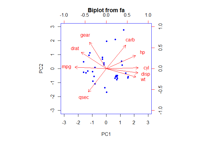
Here we can observe that hp, cyl, disp and wt contribute to PC1 with higher values. And mpg which has negative loadings is in opposite direction to PC1 with higher values. Gear and carb has higher contribution to PC2 with positive values and qsec has negative value.
Get dissimilar distance of all the variables of mtcars data as mtcars.dist
#Distance calculation
mtcars.dist<- dist(mtcars.subset)
Fit classical multi-dimensional scaling model with the mtcars.dist in 2-dimensional state as cars.mds.2d
# Fitting classical two- dimensional scaling model
cars.mds.2d<-cmdscale(mtcars.dist)
summary(cars.mds.2d)
##        V1                V2
##  Min.   :-181.07   Min.   :-139.047
##  1st Qu.:-116.69   1st Qu.: -10.373
##  Median : -43.99   Median :   2.144
##  Mean   :   0.00   Mean   :   0.000
##  3rd Qu.: 132.85   3rd Qu.:  29.375
##  Max.   : 242.81   Max.   :  52.503
Plot the cars.mds.2d and compare it with the biplot of mtcars.pca
plot(cars.mds.2d, pch = 19)
abline(h = 0, v = 0, lty =2)
mtcars.subset<-mtcars[, 1:2] %>% scale
text(cars.mds.2d, pos = 4, labels = rownames(mtcars.subset), col = "tomato")
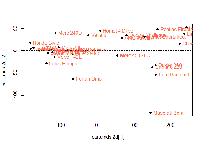
Hornet 4 Drive, Pontiac Fire bird etc lies on the positive orthant which means they have positive contribution to the first and second components. However, Lotus Europa and Ferari has opposite but highest weight component 1 and component 2.
Fit classical multi-dimensional scaling model with the mtcars.dist in 3-dimensional state as cars.mds.3d
#Fiting multi-dimensional scaling model with mtcars.dist in 3 - dimensional state
cars.mds.3d<-cmdscale(mtcars.dist, k = 3)
summary(cars.mds.3d)
##        V1                V2                 V3
##  Min.   :-181.07   Min.   :-139.047   Min.   :-6.8611
##  1st Qu.:-116.69   1st Qu.: -10.373   1st Qu.:-1.8374
##  Median : -43.99   Median :   2.144   Median : 0.8492
##  Mean   :   0.00   Mean   :   0.000   Mean   : 0.0000
##  3rd Qu.: 132.85   3rd Qu.:  29.375   3rd Qu.: 2.2806
##  Max.   : 242.81   Max.   :  52.503   Max.   : 5.0029
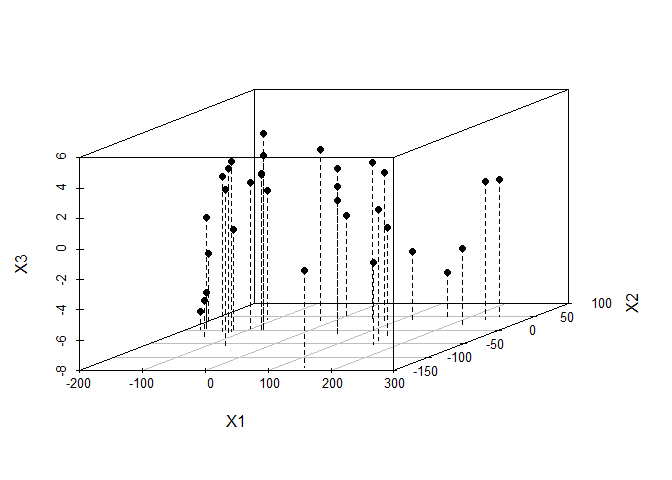
Create a 3-d scatterplot of cars.mds.3d with type = “h”, pch=20 and lty.hplot=2 and interpret it carefully
library(scatterplot3d)
cars.mds.3d <- data.frame(cmdscale(mtcars.dist, k = 3))
scatterplot3d(cars.mds.3d, type = "h", pch = 19, lty.hplot = 2)
Create a 3-d scatterplot of cars.mds.3d with type = “h”, pch=20, lty.hplot=2 and color=mtcars$cyl
library(scatterplot3d)
cars.mds.3d <- data.frame(cmdscale(mtcars.dist, k = 3))
scatterplot3d(cars.mds.3d, type = "h", pch = 19, lty.hplot = 2, color = mtcars$cyl)
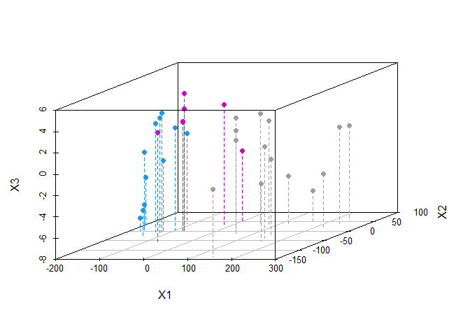
We plotted the principal components in 3- dimensional scatter plot which is distinguished by color cyl. We can use higher dimensions by changing the k argument in the cmdscale() function to a higher value for eg. k = 3 for 3 dimensuon.
Write a summary comparing PCA and MDS fits done above for mtcars data
The input to PCA is the original vectors in n-dimensional space. Similarly, input to MDS is the pairwise distances between points. PCA behaves as an algorithm but MDS is a visualization technique for any factor analysis. MDS applies PCA for the dimensionality reduction. For the mtcars, it shows that two or more but less than or equal to 5 latent features can be generated from the given dataset.


Comments