
Nepal COVID-19 data extracted from Wikipedia to fit the following models with daily deaths as dependent variable and time as independent variable
First plot the daily deaths by time and distribute the three outliers (added deaths around timeline of 400) before fitting the following models in the outlier adjusted data on training and testing datasets:
Dataset is available here.
library(readxl)
data <- read_excel("covid_tbl_final.xlsx")

str(data)
## tibble [495 x 14] (S3: tbl_df/tbl/data.frame)
##  $ SN                     : num [1:495] 1 2 3 4 5 6 7 8 9 10 ...
##  $ Date                   : POSIXct[1:495], format: "2020-01-23" "2020-01-24" ...
##  $ Confirmed_cases_total  : num [1:495] 1 1 1 1 1 1 1 1 1 1 ...
##  $ Confirmed_cases_new    : num [1:495] 1 0 0 0 0 0 0 0 0 0 ...
##  $ Confirmed _cases_active: num [1:495] 1 1 1 1 1 1 0 0 0 0 ...
##  $ Recoveries_total       : num [1:495] 0 0 0 0 0 0 1 1 1 1 ...
##  $ Recoveries_daily       : num [1:495] 0 0 0 0 0 0 1 0 0 0 ...
##  $ Deaths_total           : num [1:495] 0 0 0 0 0 0 0 0 0 0 ...
##  $ Deaths_daily           : num [1:495] 0 0 0 0 0 0 0 0 0 0 ...
##  $ RT-PCR_tests_total     : num [1:495] NA NA NA NA NA 3 4 5 5 NA ...
##  $ RT-PCR_tests_daily     : num [1:495] NA NA NA NA NA NA 1 1 0 NA ...
##  $ Test_positivity_rate   : num [1:495] NA NA NA NA NA ...
##  $ Recovery_rate          : num [1:495] 0 0 0 0 0 0 100 100 100 100 ...
##  $ Case_fatality_rate     : num [1:495] 0 0 0 0 0 0 0 0 0 0 ...
plot(data$Date, data$Deaths_total, main = "Total Deaths", xlab = "Date", ylab = "Deaths_total")
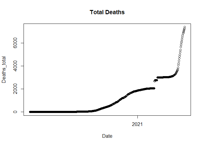
The graph shows there’s a break in between, so the trend is discontinued for some days. We plot daily deaths next to see on what date the breakage occurs.
#plotting daily deaths by time
plot(data$Date, data$Deaths_daily, main = "Daily deaths", xlab = "Date", ylab = "Daily Deaths")
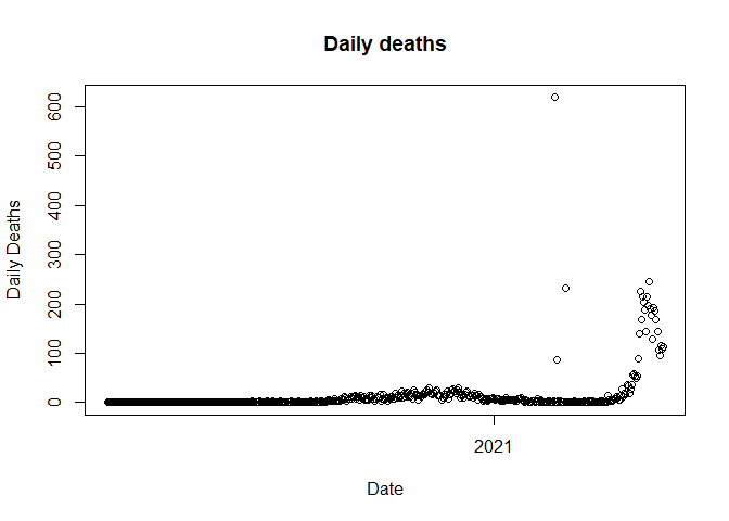
We observed three outliers in the above plot. Next, we need to identify the date on which each outlier is present.
# Identify outliers
# Value 75 has been choosed based upon the graph observation.
outliers <- data[which(data$Deaths_daily > 75), ]
head(outliers[, c("SN","Date", "Deaths_daily")])
## # A tibble: 6 x 3
##      SN Date                Deaths_daily
##   <dbl> <dttm>                     <dbl>
## 1   399 2021-02-24 00:00:00          619
## 2   401 2021-02-26 00:00:00           86
## 3   408 2021-03-05 00:00:00          232
## 4   473 2021-05-09 00:00:00           88
## 5   474 2021-05-10 00:00:00          139
## 6   475 2021-05-11 00:00:00          225
It shows there are three records during February and March that have an unusual number of deaths. This data is correct as it was the correction over past counts. However, this can’t be considered as the deaths of a single date. Thus, we need to distribute the deaths accordingly.
We use the daily percentage over the total until that date to distribute the rate proportionally.
distribute_outlier <- function(SN_value) {
#SN_value = 399

  #Create adjustment to be made
  adjustment <- data[data$SN == SN_value, ]$Deaths_daily

  # Calculate average daily deaths based on last 60 days
  avg_deaths <- ceiling(mean(data[data$SN %in% c((SN_value - 1):(SN_value - 1 - 60)),]$Deaths_daily))

  # Assign average daily deaths
  data[data$SN == SN_value, ]$Deaths_daily <- avg_deaths

  # Compute the total deaths till SN_Value
  total_deaths_399 <- sum(data[data$SN <= SN_value, ]$Deaths_daily)

  # Daily Death percent contribution till SN_Value
  daily_Death_percent <- data[data$SN <= SN_value, ]$Deaths_daily / total_deaths_399

  # Daily death distribution value
  daily_Death_distribution <- round(daily_Death_percent * (adjustment - avg_deaths))

  # Add the distribution value to all the days
  data[data$SN <= SN_value, ]$Deaths_daily = data[data$SN <= SN_value, ]$Deaths_daily + daily_Death_distribution

  # Get the remaining to be adjusted value
  additional_adjustment = (adjustment - avg_deaths) - sum(daily_Death_distribution)

  # Distribute each to the past few days
  additioal_distribution_range <- data$SN %in% c(SN_value: (SN_value -  additional_adjustment + 1))
  data[additioal_distribution_range, ]$Deaths_daily <- (data[additioal_distribution_range, ]$Deaths_daily + 1)
  return(data)
  }
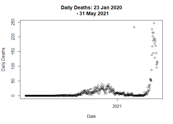
Lets plot the trend again.
data <- distribute_outlier(399)
plot(data$Date,
  data$Deaths_daily,
  main = "Daily Deaths: 23 Jan 2020
  - 31 May 2021",
  xlab = "Date",
  ylab = "Daily Deaths"
)

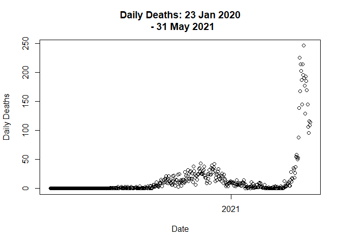
# Call distribute_outlier function to handle outlier value
# Call distribute_outlier function to handle outlier value
data <- distribute_outlier(401)

# Plot the graph on new adjustment
plot(data$Date,
  data$Deaths_daily,
  main = "Daily Deaths: 23 Jan 2020
  - 31 May 2021",
  xlab = "Date",
  ylab = "Daily Deaths"
)
# Call distribute_outlier function to handle outlier value
data <- distribute_outlier(408)

# Plot the graph on new adjustment
plot(data$Date,
  data$Deaths_daily,
  main = "Daily Deaths: 23 Jan 2020
  - 31 May 2021",
  xlab = "Date",
  ylab = "Daily Deaths"
)
total based on daily deaths.
data$new_deaths_total <- cumsum(data$Deaths_daily)
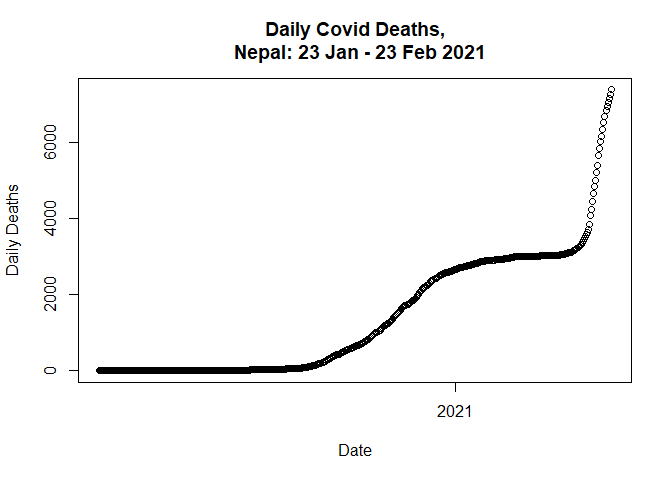
First, let’s plot the adjusted data.
plot(data$Date,
  data$new_deaths_total,
  main = "Daily Covid Deaths,
  Nepal: 23 Jan - 23 Feb 2021",
  xlab = "Date",
  ylab = "Daily Deaths")
Next, we need to do data partition into training and test set.
set.seed(13)

# Random sample for train test split
index = sample(2, nrow(data), replace = T, prob = c(0.7, 0.3))

# Get Train and test data
train.data = data[index == 1, ]
test.data = data[index == 2, ]
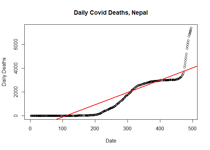
Linear Regression Model
Now lets fit a linear regression model to predict new deaths.
lm1 <- lm(new_deaths_total ~ SN, data = train.data)
summary(lm1)
##
## Call:
## lm(formula = new_deaths_total ~ SN, data = train.data)
##
## Residuals:
##    Min     1Q Median     3Q    Max
## -893.5 -472.0  -99.0  237.6 3397.2
##
## Coefficients:
##               Estimate Std. Error t value Pr(>|t|)
## (Intercept) -1125.5876    77.4326  -14.54   <2e-16 ***
## SN             10.3321     0.2727   37.88   <2e-16 ***
## ---
## Signif. codes:  0 '***' 0.001 '**' 0.01 '*' 0.05 '.' 0.1 ' ' 1
##
## Residual standard error: 738.3 on 350 degrees of freedom
## Multiple R-squared:  0.8039, Adjusted R-squared:  0.8034
## F-statistic:  1435 on 1 and 350 DF,  p-value: < 2.2e-16
Plotting linear regression
Lets plot the model.
# Plot simple linear regression model
plot(new_deaths_total ~ SN,
     data = train.data,
     main = "Daily Covid Deaths, Nepal",
     xlab = "Date",
     ylab = "Daily Deaths")
abline(lm(new_deaths_total ~ SN, data = train.data), col = "red", lwd=2)
Constructing quadratic regression model
qlm <- lm(new_deaths_total ~ poly(SN, 2, raw=T), data = train.data)
summary(qlm)
##
## Call:
## lm(formula = new_deaths_total ~ poly(SN, 2, raw = T), data = train.data)
##
## Residuals:
##      Min       1Q   Median       3Q      Max
## -1179.85  -203.82    10.23   103.66  2202.96
##
## Coefficients:
##                        Estimate Std. Error t value Pr(>|t|)
## (Intercept)           75.666058  76.479598   0.989    0.323
## poly(SN, 2, raw = T)1 -4.347558   0.716345  -6.069 3.35e-09 ***
## poly(SN, 2, raw = T)2  0.029627   0.001399  21.177  < 2e-16 ***
## ---
## Signif. codes:  0 '***' 0.001 '**' 0.01 '*' 0.05 '.' 0.1 ' ' 1
##
## Residual standard error: 489.1 on 349 degrees of freedom
## Multiple R-squared:  0.9142, Adjusted R-squared:  0.9137
## F-statistic:  1859 on 2 and 349 DF,  p-value: < 2.2e-16
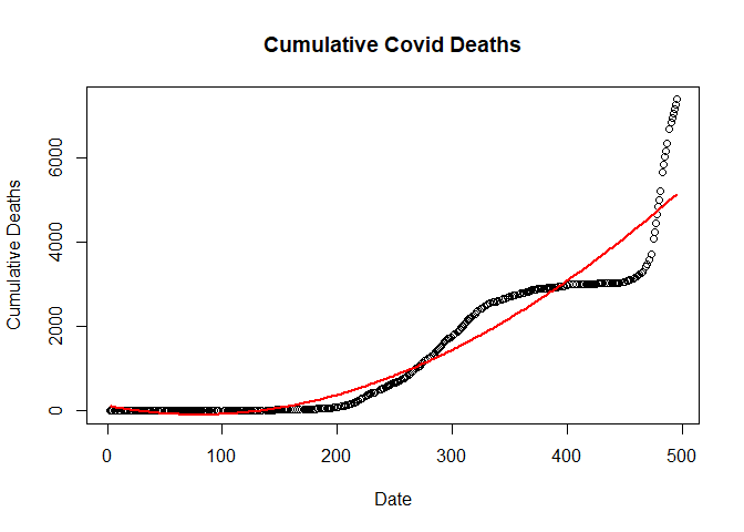
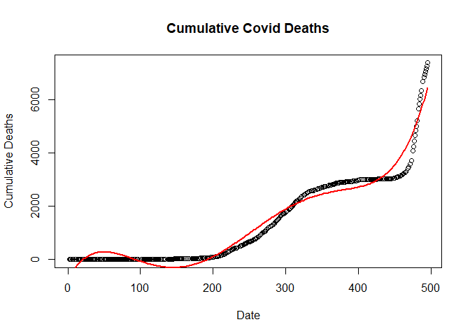
Plotting Quadratic linear model
plot(new_deaths_total ~ SN,
     data = train.data,
     main = "Cumulative Covid Deaths",
     xlab = "Date",
     ylab = "Cumulative Deaths")

lines(fitted(qlm) ~ SN, data=train.data, col="red", lwd=2)

Fitting Cubic regression Model
clm <- lm(new_deaths_total ~ poly(SN, 3, raw=T), data = train.data)
summary(clm)
##
## Call:
## lm(formula = new_deaths_total ~ poly(SN, 3, raw = T), data = train.data)
##
## Residuals:
##      Min       1Q   Median       3Q      Max
## -1168.69  -196.88     6.18    93.46  2241.65
##
## Coefficients:
##                         Estimate Std. Error t value Pr(>|t|)
## (Intercept)            1.187e+02  1.040e+02   1.142  0.25417
## poly(SN, 3, raw = T)1 -5.386e+00  1.842e+00  -2.924  0.00368 **
## poly(SN, 3, raw = T)2  3.483e-02  8.619e-03   4.042 6.54e-05 ***
## poly(SN, 3, raw = T)3 -6.955e-06  1.136e-05  -0.612  0.54072
## ---
## Signif. codes:  0 '***' 0.001 '**' 0.01 '*' 0.05 '.' 0.1 ' ' 1
##
## Residual standard error: 489.5 on 348 degrees of freedom
## Multiple R-squared:  0.9143, Adjusted R-squared:  0.9136
## F-statistic:  1237 on 3 and 348 DF,  p-value: < 2.2e-16
Plotting Cubic Regression Model
plot(new_deaths_total ~ SN,
     data = train.data,
     main = "Cumulative Covid Deaths",
     xlab = "Date",
     ylab = "Cumulative Deaths")

lines(fitted(clm) ~ SN, data=train.data, col="red", lwd=2)
Fitting Double quardatic linear regression model
dlm <- lm(new_deaths_total ~ poly(SN, 4, raw=T), data = train.data)
summary(qlm)
##
## Call:
## lm(formula = new_deaths_total ~ poly(SN, 2, raw = T), data = train.data)
##
## Residuals:
##      Min       1Q   Median       3Q      Max
## -1179.85  -203.82    10.23   103.66  2202.96
##
## Coefficients:
##                        Estimate Std. Error t value Pr(>|t|)
## (Intercept)           75.666058  76.479598   0.989    0.323
## poly(SN, 2, raw = T)1 -4.347558   0.716345  -6.069 3.35e-09 ***
## poly(SN, 2, raw = T)2  0.029627   0.001399  21.177  < 2e-16 ***
## ---
## Signif. codes:  0 '***' 0.001 '**' 0.01 '*' 0.05 '.' 0.1 ' ' 1
##
## Residual standard error: 489.1 on 349 degrees of freedom
## Multiple R-squared:  0.9142, Adjusted R-squared:  0.9137
## F-statistic:  1859 on 2 and 349 DF,  p-value: < 2.2e-16
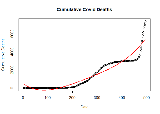
Ploting double quardatic model
plot(new_deaths_total ~ SN,
     data = train.data,
     main = "Cumulative Covid Deaths",
     xlab = "Date",
     ylab = "Cumulative Deaths")

lines(fitted(dlm) ~ SN, data=train.data, col="red", lwd=2)
Fifth order linear regression model
flm <- lm(new_deaths_total ~ poly(SN, 5, raw=T), data = train.data)
summary(flm)
##
## Call:
## lm(formula = new_deaths_total ~ poly(SN, 5, raw = T), data = train.data)
##
## Residuals:
##     Min      1Q  Median      3Q     Max
## -933.64 -227.84    7.33  253.20  944.68
##
## Coefficients:
##                         Estimate Std. Error t value Pr(>|t|)
## (Intercept)           -7.601e+02  1.072e+02  -7.092 7.48e-12 ***
## poly(SN, 5, raw = T)1  5.169e+01  4.298e+00  12.026  < 2e-16 ***
## poly(SN, 5, raw = T)2 -8.353e-01  5.312e-02 -15.724  < 2e-16 ***
## poly(SN, 5, raw = T)3  4.947e-03  2.702e-04  18.306  < 2e-16 ***
## poly(SN, 5, raw = T)4 -1.172e-05  5.986e-07 -19.583  < 2e-16 ***
## poly(SN, 5, raw = T)5  9.760e-09  4.788e-10  20.387  < 2e-16 ***
## ---
## Signif. codes:  0 '***' 0.001 '**' 0.01 '*' 0.05 '.' 0.1 ' ' 1
##
## Residual standard error: 320.4 on 346 degrees of freedom
## Multiple R-squared:  0.9635, Adjusted R-squared:  0.963
## F-statistic:  1827 on 5 and 346 DF,  p-value: < 2.2e-16
Plot of fifth order regression model
plot(new_deaths_total ~ SN,
     data = train.data,
     main = "Cumulative Covid Deaths",
     xlab = "Date",
     ylab = "Cumulative Deaths")

lines(fitted(flm) ~ SN, data=train.data, col="red", lwd=2)
KNN Regression model
library(caret)
## Warning: package 'caret' was built under R version 4.1.2

## Loading required package: ggplot2

## Loading required package: lattice
Knreg<-knnreg(new_deaths_total~SN, data = train.data)
summary(Knreg)
##         Length Class  Mode
## learn   2      -none- list
## k       1      -none- numeric
## terms   3      terms  call
## xlevels 0      -none- list
## theDots 0      -none- list
ANN-MLP regression model with 2 hidden layers with 3 and 2 neurons
Lets make a Multi Layer Perceptron with 2 hidden layers and 3 and 2 neurons.
library(neuralnet)
## Warning: package 'neuralnet' was built under R version 4.1.2
ann<- neuralnet(Deaths_total ~ SN,
               data=train.data,
               hidden = c(3,2),
               linear.output=F)

plot(ann)
Selecting the best model with lowest RMSE on the test data
# Evaluate Linear Model
pred = predict(lm1, test.data)
lm1_RMSE <- RMSE(pred, test.data$new_deaths_total)

# Evaluate Quadratic Linear Model
pred = predict(qlm, test.data)
qlm_RMSE<- RMSE(pred, test.data$new_deaths_total)

# Evaluate Cubic Linear Model
pred = predict(clm, test.data)
clm_RMSE<- RMSE(pred, test.data$new_deaths_total)

# Evaluate Double Quadratic Linear Model
pred = predict(dlm, test.data)
dlm_RMSE <- RMSE(pred, test.data$new_deaths_total)

# Evaluate Fifth Order Polynomial Linear Model
pred = predict(flm, test.data)
flm_RMSE <- RMSE(pred, test.data$new_deaths_total)

# Evaluate KNN Model
pred = predict(Knreg, data.frame(test.data))
Knreg_RMSE <- RMSE(pred, test.data$new_deaths_total)

# Evaluate Neural Network Model
nn.results <- compute(ann, test.data)
ann_RMSE <- RMSE(nn.results$net.result, test.data$new_deaths_total)

# Add all calculated RMSE to the data frame and print the result
RMSE_data <- data.frame(
  "Linear Model" = lm1_RMSE,
  "Quadratic Model " = qlm_RMSE,
  "Cubic Model" = clm_RMSE,
  "Double Quadratic Model" = dlm_RMSE,
  "Fifth Order Linear Model" = flm_RMSE,
  "K Nearest Neighbour" = Knreg_RMSE,
  "Artificial Neural Network" = ann_RMSE
  )
print(RMSE_data)
##   Linear.Model Quadratic.Model. Cubic.Model Double.Quadratic.Model
## 1     563.3899         455.9349    451.4325               454.3285
##   Fifth.Order.Linear.Model K.Nearest.Neighbour Artificial.Neural.Network
## 1                 318.4373            19.13961                  2027.773
It seems KNN gives the best result.


Comments