R Exercise: Social Network Analysis

Social Network Analysis

Definition

Social networks are simply networks of social interactions and personal relationships. Think about our group of friends and how we got to know them. Maybe we met them while ago from our schooling, or maybe we met them through a hobby or through our community. In fact, 72% of all Internet users are active on social media today, including in social interactions and developing personal relationships. However, to understand about social networks, we only don’t need to go through internet or social media, they may come in variety of form in our daily life.

Social Network Analysis

Social network analysis (SNA), also known as network science, is a field of data analytics that uses networks and graph theory to understand social structures. We can see network around us such as road network, online network, network of social media such as facebook, twitter etc. Learning SNA allow us to explore insight of various data sources.

SNA Graph

We all are familier about the graph which simply the collection of non zero vertex and edge. In order to build SNA graphs, two key components are required actors and relationships. Here, actors represents the vertex and relationship means the edge between two actors. Let us write SNA graph in R code. To do this, we should have igraph package already install in our R or R studio.

library(igraph)

## 
## Attaching package: 'igraph'

## The following objects are masked from 'package:stats':
## 
##     decompose, spectrum

## The following object is masked from 'package:base':
## 
##     union

g <- graph(c(1,2))
plot(g)

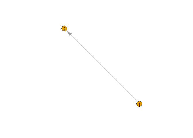
In figure, we can see the directed graph from node 1 to node 2. From above graph, it is also clear that by default it gives directed graph. In above figure we can not clearly see node and edge so let’s increase its size and give different color to the node.

plot(g,
vertex.color = 'green',
vertex.size = 40,
edge.color ='red',
edge.size = 20)

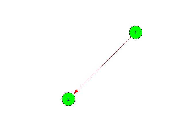
Now we change the node color and node font size. Add more node on graph for this we follow the following code.

g <- graph(c(1,2,2,3,3,4,4,1))
plot(g,
     vertex.color = 'green',
     vertex.size =40,
     edge.color = 'red',
     edge.size = 20)

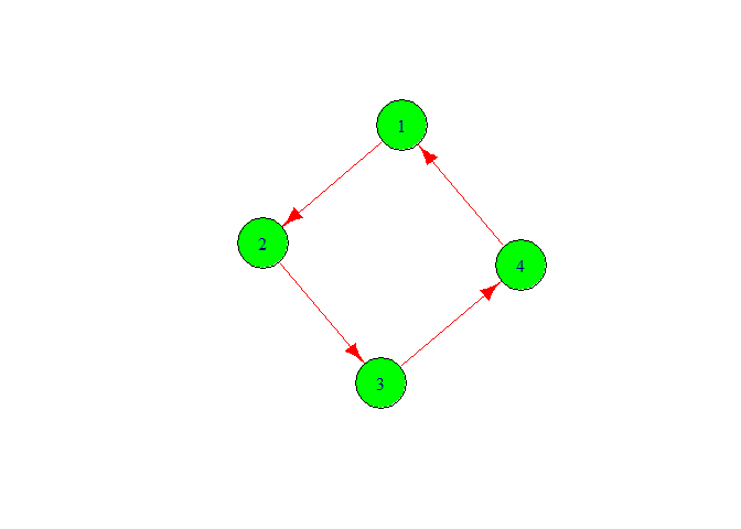
We got the graph with four vertex 1,2,3,4. Here, we also got directed graph. Let’s make it for this we need to write directed is false.

g <- graph(c(1,2,2,3,3,4,4,1),directed = FALSE)
plot(g,
     vertex.color = 'green',
     vertex.size =40,
     edge.color = 'red',
     edge.size = 20)

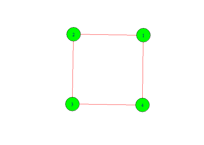
We got our desirable type of graph. Now let’s move forword. We can give the number of vertex with out writing them for this look following code.

g <- graph(c(1,2,2,3,3,4,4,1), 
directed = F, n=7)
plot(g,
     vertex.color = 'green',
     vertex.size =40,
     edge.color = 'red',
     edge.size = 20)

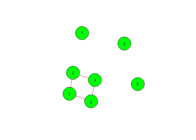
In above graph we have given seven vertex numbers. Among them we can see three isolated nodes. The reason to come isolated node is that we did not specify the edge or relationship between them. Also from graph we can make sense that this is not directed graph.

Adjacency Matrix

Let’s see what will happen if we type only g[].

g[]

## 7 x 7 sparse Matrix of class "dgCMatrix"
##                   
## [1,] . 1 . 1 . . .
## [2,] 1 . 1 . . . .
## [3,] . 1 . 1 . . .
## [4,] 1 . 1 . . . .
## [5,] . . . . . . .
## [6,] . . . . . . .
## [7,] . . . . . . .

This gives us the 7 by 7 adjacency matrix. Adjancency matrix is matix where we give 1 if there is edge between two vertex if not then we give 0. But in above matrix it gave simply . instead of zero.

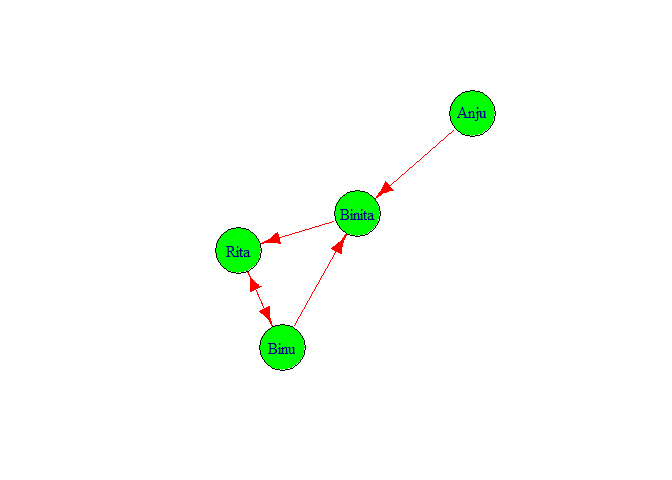
Let us try to build our graph by keeping text data in place of number.

g1 <-
graph(c("Binu","Binita","Binita","Rita"
,"Rita","Binu","Binu","Rita", "Anju", 
"Binita"))
plot(g1,
vertex.color = "green",
vertex.size = 40,
edge.color = "red",
edge.size = 5)

If we want to check the features of g1 we simply type g1 and press control and enter key. We got following output.

g1

## IGRAPH d030509 DN-- 4 5 -- 
## + attr: name (v/c)
## + edges from d030509 (vertex names):
## [1] Binu  ->Binita Binita->Rita   Rita  ->Binu   Binu  ->Rita   Anju  ->Binita

It showed that in graph there are 4 nodes 5 edges. And edges are directed from Binu ->Binita, Binita->Rita, Rita ->Binu, Binu ->Rita, Anju ->Binita.

Degree

Degree means numbers of connection to each node. Let’s check the degree of graph g1. To check degree we can do degree(g1) or degree(g1, mode='all').

degree(g1) 

##   Binu Binita   Rita   Anju 
##      3      3      3      1

Degree of Binu is 3 similarly Anju has degree 1.

degree(g1, mode='all')

##   Binu Binita   Rita   Anju 
##      3      3      3      1

Diameter

Diameter means number of edged inside and outside of SND. Now, let’s check the diameter of graph.

diameter(g1, directed = F, weights = 
NA)

## [1] 2

We got two diameter. i.e Anju <- Binita <- Rita, Anju <- Binita <- Binu.

Edge density

Edge density means ecount(g1)/(vcount(g1)*(vcount(g1) -1)). We can calculate it from following code.

edge_density(g1, loops = F)

## [1] 0.4166667

We got the value of edge density 0.4166667.

Reciprocity

Total edges = 5

Tied edges = 2

Reciprocity = 2/5 = 0.4

reciprocity(g1)

## [1] 0.4

Closeness

Now getting closeness of graph.

closeness(g1, mode = "all", weights = NA)

##      Binu    Binita      Rita      Anju 
## 0.2500000 0.3333333 0.2500000 0.2000000

From above result we can see that Binita is closest to the others three persons and Anju is farthest from other three persons.

Betweenness

Let’s calculate between of g1

betweenness(g1, directed = T, weights = NA)

##   Binu Binita   Rita   Anju 
##      1      2      2      0

Binita and Rita has 2 inner edge similarly Binu has one inner edge and Anju has no inner edge.

Edge Betweenness

For every pair of vertices in a connected graph, there exists at least one shortest path between the vertices.

edge_betweenness(g1, directed = T, weights = NA)

## [1] 2 4 4 1 3

SNA in TwitterData

Here I have loadedTwitterdata from my local machine.

load("F:/MDS R/termDocMatrix.rdata")

m<- as.matrix(termDocMatrix)
termM <- m %*% t(m)
termM[1:10,1:10]

##               Terms
## Terms          analysis applications code computing data examples introduction
##   analysis           23            0    1         0    4        4            2
##   applications        0            9    0         0    8        0            0
##   code                1            0    9         0    1        6            0
##   computing           0            0    0        10    2        0            0
##   data                4            8    1         2   85        5            3
##   examples            4            0    6         0    5       17            2
##   introduction        2            0    0         0    3        2           10
##   mining              4            7    3         1   50        5            3
##   network            12            0    1         0    0        2            2
##   package             2            1    0         2   12        2            0
##               Terms
## Terms          mining network package
##   analysis          4      12       2
##   applications      7       0       1
##   code              3       1       0
##   computing         1       0       2
##   data             50       0      12
##   examples          5       2       2
##   introduction      3       2       0
##   mining           64       1       6
##   network           1      17       1
##   package           6       1      27

Now we have built a term-term adjacency matrix, where the rows and columns represents terms, and every entry is the number of co-occurrences of two terms. Next we can build a graph with graph.adjacency() from package igraph.

g <- graph.adjacency(termM,weighted = T,mode = 'undirected')
g

## IGRAPH d066e18 UNW- 21 151 -- 
## + attr: name (v/c), weight (e/n)
## + edges from d066e18 (vertex names):
##  [1] analysis    --analysis     analysis    --code        
##  [3] analysis    --data         analysis    --examples    
##  [5] analysis    --introduction analysis    --mining      
##  [7] analysis    --network      analysis    --package     
##  [9] analysis    --positions    analysis    --postdoctoral
## [11] analysis    --r            analysis    --research    
## [13] analysis    --series       analysis    --slides      
## [15] analysis    --social       analysis    --time        
## + ... omitted several edges

Here we have built graph on termDocMatrix. In result we can see the edges between different dodes.

g <- simplify(g)
g

## IGRAPH d06a87e UNW- 21 130 -- 
## + attr: name (v/c), weight (e/n)
## + edges from d06a87e (vertex names):
##  [1] analysis    --code         analysis    --data        
##  [3] analysis    --examples     analysis    --introduction
##  [5] analysis    --mining       analysis    --network     
##  [7] analysis    --package      analysis    --positions   
##  [9] analysis    --postdoctoral analysis    --r           
## [11] analysis    --research     analysis    --series      
## [13] analysis    --slides       analysis    --social      
## [15] analysis    --time         analysis    --tutorial    
## + ... omitted several edges

Function simplify() in igraph handly removes self-loops from a network. We can see in previous graph there are 151 edges in second graph there are only 130 edges. Hence there are 21 self loops they are omitted from the graph.

Check Degree of graph and nodes of the graph.

V(g)$label <- V(g)$name
V(g)$label

##  [1] "analysis"     "applications" "code"         "computing"    "data"        
##  [6] "examples"     "introduction" "mining"       "network"      "package"     
## [11] "parallel"     "positions"    "postdoctoral" "r"            "research"    
## [16] "series"       "slides"       "social"       "time"         "tutorial"    
## [21] "users"

V(g)$degree <- degree(g)
V(g)$degree

##  [1] 17  6  9  9 18 14 12 20 14 13  8  7  8 17  9 11 15 11 11 16 15

We found degree of graph is 20.

Histogram on the basis of degree

hist(V(g)$degree, breaks = 100,col = 'green', main = "Frequency Of Degree", 
     xlab = " Degree of vertices", ylab = " Frequency")

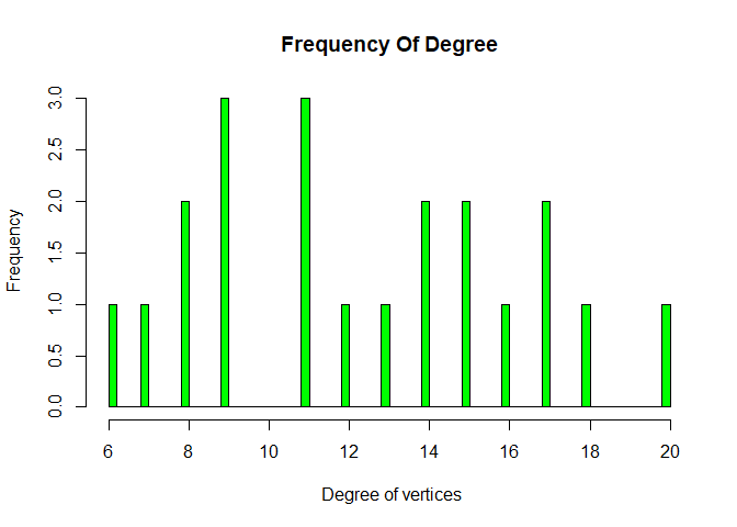
We can see most of nodes have degree 9 and 11. We all khow what is degree of graph, number of edges that are incident to the node is called degree of graph.

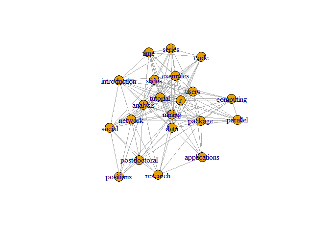
Let’s Plot Graph on the Data.

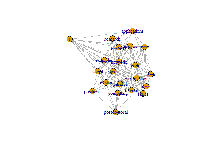
Let’s set set.seed(3952). Where set.seed gives same sample with the same seed value.

set.seed(3952)

layout1 <- layout.fruchterman.reingold(g)

plot(g, layout=layout1)

A different layout can be generated with the first line of code below. The second line produces an interactive plot, which allows us to manually rearrange the layout

plot(g, layout=layout.kamada.kawai)

## Make it better.

V(g)$label.cex <- 2.2 * V(g)$degree / max(V(g)$degree)+ .2

V(g)$label.color <- rgb(0, 0, .2, .8)

V(g)$frame.color <- NA

egam <- (log(E(g)$weight)+.4) / max(log(E(g)$weight)+.4)

E(g)$color <- rgb(.5, .5, 0, egam)

E(g)$width <- egam
# plot the graph in layout1

plot(g, layout=layout1)

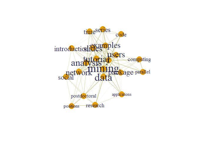
Here size of words appear according to their degree. From graph we can clearly see that node mining has maximum degree.

Community detection

Communities are seen as groups, clusters, coherent subgroups, or modules in different fields; community detection in a social network is identifying sets of nodes in such a way that the connections of nodes within a set are more than their connection to other network nodes.

comm <- cluster_edge_betweenness(g)

## Warning in cluster_edge_betweenness(g): At community.c:461 :Membership vector
## will be selected based on the lowest modularity score.

## Warning in cluster_edge_betweenness(g): At community.c:468 :Modularity
## calculation with weighted edge betweenness community detection might not make
## sense -- modularity treats edge weights as similarities while edge betwenness
## treats them as distances

plot(comm,g)

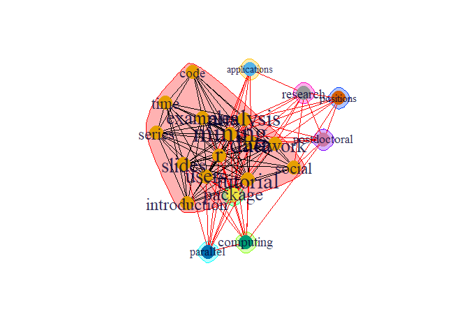
There are dense connection within the group within the community the connection is sparse.

prop <- cluster_label_prop(g)
plot(prop, g)

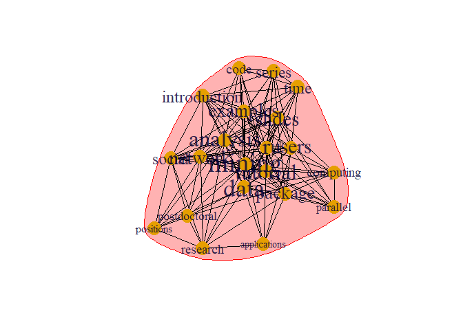
This is different type of algorithms to detect community which is different from previous one.

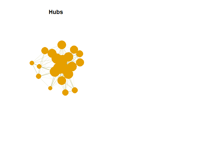
Hubs

Nodes with most outer edges. We need to find hub score.

hs <- hub_score(g,weights = NA)$vector
hs

##     analysis applications         code    computing         data     examples 
##    0.9047777    0.3589289    0.5606314    0.5223206    0.9065063    0.8195307 
## introduction       mining      network      package     parallel    positions 
##    0.7307838    1.0000000    0.7483791    0.7210610    0.4939614    0.3733995 
## postdoctoral            r     research       series       slides       social 
##    0.4095660    0.9147530    0.4481802    0.6761093    0.8510808    0.6018664 
##         time     tutorial        users 
##    0.6761093    0.8899001    0.8342594

Authority

Nodes with most inner edges. We need to find authority score

as <- authority_score(g, weights = NA)$vector
as

##     analysis applications         code    computing         data     examples 
##    0.9047777    0.3589289    0.5606314    0.5223206    0.9065063    0.8195307 
## introduction       mining      network      package     parallel    positions 
##    0.7307838    1.0000000    0.7483791    0.7210610    0.4939614    0.3733995 
## postdoctoral            r     research       series       slides       social 
##    0.4095660    0.9147530    0.4481802    0.6761093    0.8510808    0.6018664 
##         time     tutorial        users 
##    0.6761093    0.8899001    0.8342594

Hub in Plot

par(mfrow = c(1,2))
plot(g,vertex.size= hs*50, main = "Hubs",
     vertex.label = NA,
     vertex.colour = rainbow(50))

Authority in Plot

plot(g,vertex.size= as*30, main = "Authorities",
     vertex.label = NA,
     vertex.colour = rainbow(50))

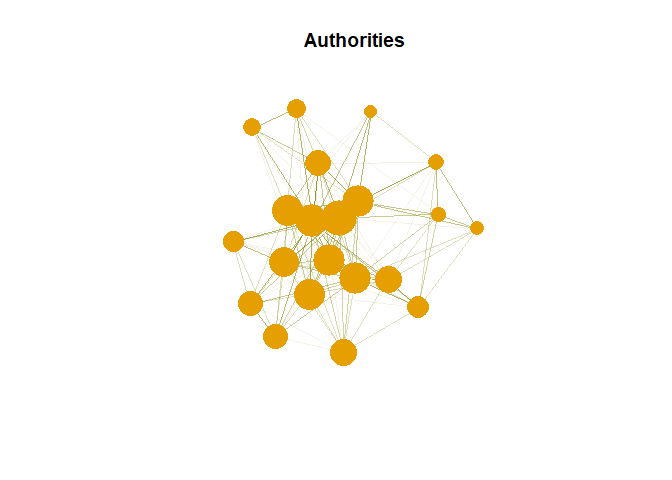
Hub are expected to contain large number of outgoing link. And authority are expected to contain large number of incoming link from hubs.

Application of SNA in Real World

Social network analysis can provide information about the reach of gangs, the impact of gangs, and gang activity. The approach may also allow we to identify those who may be at risk of gang-association and/or being exploited by gangs.