
Gradient Descent
Gradient Descent is one of the most widely used optimizers for updating model parameters in machine learning. It works by calculating the gradient of the error with respect to the parameters and adjusting the parameters to minimize the error. However, the specific rule for updating parameters can vary, leading to different variants of Gradient Descent. These variants, such as Stochastic Gradient Descent (SGD), Mini-batch Gradient Descent, and Adam, offer unique advantages and trade-offs in terms of speed, stability, and convergence efficiency, depending on the problem being addressed.
Mini- Batch Gradient Decent
It is the simplest algorithm, where we update parameters in each batch. In each batch there will be number of examples.
Import necessary module
pandas: Working for DataFramenumpy: For array operationmatplotlib: for visualization
Read csv data in pandas Dataframe
import pandas as pd
import numpy as np
import matplotlib.pyplot as plt

df = pd.read_csv('F:/MDS-Private-Study-Materials/Second Semester/Applied Machine Learning/data.csv')
df.head()
df.shape
(100, 2)
df.head()
| x | y | |
|---|---|---|
| 0 | 32.502345 | 31.707006 |
| 1 | 53.426804 | 68.777596 |
| 2 | 61.530358 | 62.562382 |
| 3 | 47.475640 | 71.546632 |
| 4 | 59.813208 | 87.230925 |
Split Data
We split data into train set and test set in the ratio of 70% to 30%
split = int(len(df)*0.7)
train_x, test_x = df[:split].x , df[split:].x
train_y, test_y = df[:split].y , df[split:].y

len(train_x)
70
Create class Mini_batch_gradient_decent
Create method create_batch inside class which takes train data, test data and batch_sizes as parameter. We create mini_batches = [] to store the value of each batches. data = np.stack((train_x,train_y), axis=1) function join train_x and train_y into first dimension. Number of batches is row divide by batches size. We use for loop in the range of no_of_batches. ` mini_batch = data[i * batch_size: (i+1)* batch_size] which create mini batch from 0 to if we give batch_size 10 upto 10 in the next iteration mini_batch will be 10 to 20 and so on. If number of row is not exactly divided by batch size then there will be data remain outside of batch so we will do train_x.shape[0]%batch_size != 0` then we will keep all the batch data into mini_batches list by using append function. In first column we kept x values and in second column we kept y values. Finally we return mini_batches.
class Mini_batch_gradient_decent:
    def create_batch(self,train_x, train_y, batch_size):

        mini_batches = []
        data = np.stack((train_x,train_y), axis=1)

        no_of_bathches = train_x.shape[0]//batch_size

        for i in range(no_of_bathches):

            mini_batch = data[i * batch_size: (i+1)* batch_size]

            mini_batches.append((mini_batch[:,0],mini_batch[:,1]))
        if train_x.shape[0]%batch_size != 0:
            mini_batchi = data[i* batch_size:]
            mini_batches.append((mini_batch[:,0],mini_batch[:,1]))
        return mini_batches
Model Fitting
The function fit() is defined, with the parameters train x, train y, alpha, epochs, batch size. Then we set the slope and intercept values to 1 and 1, respectively. In addition, the letter l denotes the total number of observations. In the range of epochs, we used for loop. The batch function is then called, as explained in the previous cell block. We utilize the for loop in batches again, this time with xb indicating batch x values and yb indicating batch y values, and then we reshape the xb and yb. We can take all rows but only one column with xb.reshape(-1,1). The same is true for y. Define the linear regression projected value now. The mean square error is next defined, and finally, the mean square error is calculated.
import time
class Mini_batch_gradient_decent:

    def create_batch(self,train_x, train_y, batch_size):
        mini_batches = []
        data = np.stack((train_x,train_y), axis=1)

        no_of_bathches = train_x.shape[0]//batch_size

        for i in range(no_of_bathches):

            mini_batch = data[i * batch_size: (i+1)* batch_size]

            mini_batches.append((mini_batch[:,0],mini_batch[:,1]))
        if train_x.shape[0]%batch_size != 0:
            mini_batchi = data[i* batch_size:]
            mini_batches.append((mini_batch[:,0],mini_batch[:,1]))
        return mini_batches

    def fit(self, train_x, train_y, alpha, epochs, batch_size, show_every=1000):


        self.m = np.random.randn(1,1)
        self.c = np.random.randn(1,1)

        l = len(train_x)

        for i in range(epochs):

            batches = self.create_batch(train_x, train_y, batch_size)

            t1=time.time()
            for batch in batches:

                xb = batch[0]
                yb = batch[1]
                n = len(xb)

                xb = xb.reshape(-1,1)
                #print(xb)
                yb = yb.reshape(-1,1)
                #print(yb)

                delta_intercept = None
                delta_slope = None
                yp = np.dot(xb, self.m)+self.c


                err=(0.5/n) * np.sum((yb-yp)**2)

                delta_intercept = -(1/n) * np.sum(yb-yp)
                delta_slope = -(1/n) * np.sum((yb-yp)*xb)


                self.m = self.m - alpha* (delta_slope)
                self.c = self.c - alpha * (delta_intercept)
            if i% show_every==0:
                print(f"Iteration {i}: Error: {err}, time = {(time.time()-t1)/60}")


    def slope_intercept(self):
        print(f"Slope is {self.m[0][0]}")
        print(f"Intercept is {self.c[0][0]}")

    def predict(self, test_x):
        test_x = test_x.reshape(test_x.shape[0],1)
        self.m = self.m.reshape((self.m.shape[0],self.m.shape[0]))
        result = np.dot(test_x,self.m) + self.m
        return result
We have also defined functions for slope and intercept as well as prediction in the code block below. The prediction function takes the value of test x and returns the result.
Function call
We use our own dummy data to invoke the function here. The goal of using this data is to determine whether or not our model is functioning appropriately. Our model is looking fantastic. Our model should give us a value for c 1 and a value for m 1500, and we can see that it does.
mgd = Mini_batch_gradient_decent()

mgd.fit(np.arange(1,500)/500, 1+3*np.arange(1,500),0.01,5000, 32)
Iteration 0: Error: 759204.9669527125, time = 2.5204817454020183e-05
Iteration 1000: Error: 6.181828420803425e-05, time = 0.0
Iteration 2000: Error: 4.176020605988289e-14, time = 0.0
Iteration 3000: Error: 7.235164641068069e-23, time = 1.659393310546875e-05
Iteration 4000: Error: 7.235164641068069e-23, time = 1.1889139811197917e-05
mgd.slope_intercept()
Slope is 1499.999999999971
Intercept is 1.0000000000151974
It seems that our model did pretty well. Lets try on our original data.
mgd.fit(train_x, train_y,0.0001,5000, 16)
Iteration 0: Error: 273.93246976150095, time = 8.436044057210286e-06
Iteration 1000: Error: 47.568936899285255, time = 1.6987323760986328e-05
Iteration 2000: Error: 47.47580315198226, time = 1.659393310546875e-05
Iteration 3000: Error: 47.38452227067236, time = 0.0
Iteration 4000: Error: 47.29505307924061, time = 1.6828378041585285e-05
Lets see the fitted model on our data.
plt.scatter(train_x, train_y)
plt.plot(train_x, np.dot(train_x.to_numpy().reshape(-1,1), mgd.m)+mgd.c, c="r")
plt.show()
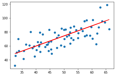
Since the data points wee scattered, the best linear line goes from the middle.
Batch gradient decent
The function define gradient decent() takes the parameters train x, y true, epochs, learning rate. Set the value of m and c to 1. Make an empty list to keep track of the number of errors in each iteration. The entire length of observations is denoted by the letter l. Use for loops in the period range. Define xb and yb from train x and y true, respectively, where .reshape(-1,1) indicates that we can choose any rows but only one column. Define yp now. Then define what square mistake implies. Then, for both slope and intercept, determine the gradient. After that, change the values of the parameters m and c. Finally, we provided dummy data before testing our model on real data to ensure that it was working properly.
def batch_gradient_decent(train_x, y_true, epochs, learning_rate = 0.001, show_every=1000):

    m = np.random.randn(1,1)
    c = np.random.randn(1,1)
    l = len(train_x)
    errs = []

    for i in range(epochs):
        t1= time.time()

        xb = train_x.reshape(-1,1)
        yb = y_true.reshape(-1,1)

        delta_intercept = None
        delta_slope = None
        yp = np.dot(xb, m)+c

        n = len(xb)
        err=(0.5/n) * np.sum((yb-yp)**2)

        delta_intercept = -(1/n) * np.sum(yb-yp)
        delta_slope = -(1/n) * np.sum((yb-yp)*xb)

        m = m - learning_rate * delta_slope
        c = c- learning_rate* delta_intercept
        errs.append(err)
        if i%show_every==0:
            print(f"Iteration {i}: Error: {err}, time: {(time.time()-t1)/60}")
    return m, c, errs
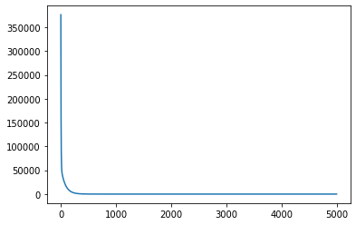
Lets use simple example again.
m,c,errs=batch_gradient_decent(np.arange(1,500)/500, 1+3*np.arange(1,500),5000,0.1)
Iteration 0: Error: 377387.06815160357, time: 1.781781514485677e-05
Iteration 1000: Error: 0.11260563371092129, time: 0.0
Iteration 2000: Error: 2.2137776134628694e-07, time: 0.0
Iteration 3000: Error: 4.3521897372030944e-13, time: 0.0
Iteration 4000: Error: 8.557543667725901e-19, time: 1.662572224934896e-05
m
array([[1500.]])
Which is obvious as we have made data that way.
In our case error is decreasing rapidly in some iterations and decreasing gradually in last some iterations.
plt.plot(errs)
[<matplotlib.lines.Line2D at 0x24e996bc790>]
Using original Data
m,c,errs = batch_gradient_decent(train_x.to_numpy(), train_y.to_numpy(),5000,0.0001)

plt.plot(errs)
Iteration 0: Error: 2621.494652507566, time: 0.0
Iteration 1000: Error: 58.74680115227563, time: 0.0
Iteration 2000: Error: 58.745205635524144, time: 1.659393310546875e-05
Iteration 3000: Error: 58.743620912278544, time: 0.0
Iteration 4000: Error: 58.74204690952185, time: 0.0


[<matplotlib.lines.Line2D at 0x24e994eb730>]
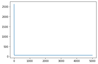
It did pretty well.
Stochastic Gradient Decent
if we keep value of batch_size = 1 in mini-batch gradient decent then it becomes stochastic gradient decent.
class Stochastic_gradient_decent:
    def create_batch(self,train_x, train_y, batch_size):
        mini_batches = []
        data = np.stack((train_x,train_y), axis=1)

        no_of_bathches = train_x.shape[0]//batch_size

        for i in range(no_of_bathches):

            mini_batch = data[i * batch_size: (i+1)* batch_size]

            mini_batches.append((mini_batch[:,0],mini_batch[:,1]))
        if train_x.shape[0]%batch_size != 0:
            mini_batchi = data[i* batch_size:]
            mini_batches.append((mini_batch[:,0],mini_batch[:,1]))
        return mini_batches

    def fit(self, train_x, train_y, alpha, epochs, batch_size, show_every=1000):


        self.m = np.random.randn(1,1)
        self.c = np.random.randn(1,1)

        l = len(train_x)
        self.errs = []
        for i in range(epochs):

            batches = self.create_batch(train_x, train_y, batch_size)

            t1=time.time()
            for batch in batches:

                xb = batch[0]
                yb = batch[1]
                n = len(xb)

                xb = xb.reshape(-1,1)
                #print(xb)
                yb = yb.reshape(-1,1)
                #print(yb)

                delta_intercept = None
                delta_slope = None
                yp = np.dot(xb, self.m)+self.c


                err=(0.5/n) * np.sum((yb-yp)**2)

                delta_intercept = -(1/n) * np.sum(yb-yp)
                delta_slope = -(1/n) * np.sum((yb-yp)*xb)


                self.m = self.m - alpha* (delta_slope)
                self.c = self.c - alpha * (delta_intercept)
                self.errs.append(err)
            if i%show_every==0:
                print(f"Iteration {i}: Error: {err}, time = {(time.time()-t1)/60}")


    def slope_intercept(self):
        print(f"Slope is {self.m[0][0]}")
        print(f"Intercept is {self.c[0][0]}")

    def predict(self, test_x):
        test_x = test_x.reshape(test_x.shape[0],1)
        self.m = self.m.reshape((self.m.shape[0],self.m.shape[0]))
        result = np.dot(test_x,self.m) + self.m
        return result
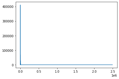
Again lets use simple example.
mgd = Stochastic_gradient_decent()

err = mgd.fit(np.arange(1,500)/500, 1+3*np.arange(1,500),0.01,5000, 1)
Iteration 0: Error: 7859.2012987632725, time = 0.0008223692576090495
Iteration 1000: Error: 6.462348535570529e-23, time = 0.00018201271692911783
Iteration 2000: Error: 6.462348535570529e-23, time = 0.0001661062240600586
Iteration 3000: Error: 6.462348535570529e-23, time = 0.000166932741800944
Iteration 4000: Error: 6.462348535570529e-23, time = 0.00018284320831298828
Lets see parameters and error.
mgd.m, mgd.c
(array([[1500.]]), array([[1.]]))
plt.plot(mgd.errs)
plt.show()
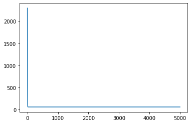
Momentum Gradient Descent
In ordinary GD, the weight or parameter is updated based on the gradient of current step only but in the Momentum, we will update parameter based on this and previous step. We will take only little fraction of the previous gradient. While typical GD stuck in local minima, Momentum provides extra push to get out of it.
def momentum_batch_gradient_decent(train_x, y_true, epochs,
                                   learning_rate = 0.001, momentum_rate=0.0001, show_every=1000):
    m = np.random.randn(1,1)
    c = np.random.randn(1,1)
    l = len(train_x)

    pds = 0
    pdi = 0
    errs = []

    for i in range(epochs):

        xb = train_x.reshape(-1,1)
        yb = y_true.reshape(-1,1)

        delta_intercept = None
        delta_slope = None
        yp = np.dot(xb, m)+c

        n = len(xb)
        err=(0.5/n) * np.sum((yb-yp)**2)

        delta_intercept = -(1/n) * np.sum(yb-yp)
        delta_slope = -(1/n) * np.sum((yb-yp)*xb)

        if i%show_every==0:
            print(f"Iteration {i}: Error: {err}")

        m = momentum_rate*pds+ m - learning_rate * delta_slope
        c = momentum_rate*pdi+c- learning_rate* delta_intercept

        pds = delta_slope
        pdi = delta_intercept
        errs.append(err)

    return m, c, errs
m,c,errs = momentum_batch_gradient_decent(train_x.to_numpy(), train_y.to_numpy(), 5000, 0.0001, 0.00001)
Iteration 0: Error: 2299.3333871682066
Iteration 1000: Error: 58.997090247292114
Iteration 2000: Error: 58.99412941821364
Iteration 3000: Error: 58.99118662197093
Iteration 4000: Error: 58.98826174873571
plt.plot(errs)
plt.show()
Comparison Between Three Gradient decent in terms of time
- Batch-gradient decent and mini-batch-gradient decent are faster as compare to stochastic gradient decent.
- In contrast to the accuracy and space, stochastic performs better.


Comments