Logistic Regression from Scratch in Python: Exploring MSE and Log Loss

Logistic Regression From Scratch

Hello everyone, here in this blog we will explore how we could train a logistic regression from scratch. We will start from mathematics and gradually implement small chunks into our code.

Import Necessary Module

• pandas : Working for DataFrame
• numpy : For array operation
• matplotlib : For visualization
• time : function creates a valid Excel time based with supplied values for hour, minute, and second

import numpy as np
import matplotlib.pyplot as plt
import pandas as pd
import time

Let’s create the function whose name is logistic which takes x and m as parameter. x is input data and m is slope. Function returns \(\frac{1}{1+ e^{-s}}\) as output. Where $ s = m.x $.

For any (multi) linear equation with W as slopes, b as intercepts and X as inputs, the output y can be written as,

\[y = XW^T+b \\\]

Or alternatively,

\[y = \begin{bmatrix} 1 && x_{01} && x_{02} && ... && x_{0j} \\ 1 && x_{11} && x_{12} && ... && x_{1j} \\ .. && .. && .. && ... && .. \\ 1 && x_{i1} && x_{i2} && ... && x_{ij} \end{bmatrix} * \begin{bmatrix} b \\ w_1 \\ .. \\ w_j \end{bmatrix}\]

Where 1s in the first column of the first part of multiplication represents the values of input which will be multiplied with bias.

def logistic(x, m):
    x = np.dot(x, m)
    yp = 1/(1+np.exp(-x))
    return yp

Also, let’s make function log_loss which take y_true and y_predict as a parameter and return \(yt* log(yp) -(1-yt) * log(1-yp)\) which is log_loss function of logistic regression.

def log_loss(yt, yp):
    return -yt * np.log(yp) - (1-yt)* np.log(1-yp)

Gradient Descent as MSE’s Gradient and Log Loss as Cost Function

Here we make gradient descent function which take X, Y, epochs and learning rate as a parameter.

    X = X.reshape(-1, X.shape[-1])
    Y = Y.reshape(-1, 1)
    

Here reshape function is used to give new shape to the array. Inside reshape function reshape(-1, x.shape[-1]) means take any rows possible but make sure column is equal to X.shape[-1]. Which simply is making sure input X has number of features equals to the number of columns.

    m = np.vstack([np.zeros(Y.shape[-1]), np.zeros((X.shape[-1],1))])
    
    X = np.hstack([np.ones((X.shape[0], 1)), X])
    

len(x) gives the length of our observation. We create list err= [] to keep error value come from each iterations. Use for loop in epochs. Yp is the predicted value for logistic regression which is obtain by calling logistic() function and error is calculated from log_loss() function then we calculate the mean of error. Here we use tm variable which means temporary mean then we used for loop which is run on len(m) inside it, we calculate grad which is gradient of parameter.

Mathematically,

\[E = \frac{1}{2m}\sum(yp- yt)^2\]

Skipping summation sign as for calculating derivative.

\(\frac{d(E)}{dw} = \frac{1}{2m}. 2.(y-yp).\frac{d(y-yp)}{dw}\) \(=\frac{1}{n}.{y-yp}.\frac{d(y-yp)}{d(yp)}.\frac{d(yp)}{dw}\)

also,

\[y_p= \frac{1}{1+e^{-S}}\]

and

\[S = X.W^T + b\]

and \(\frac{1}{1+e^{-s}} = \frac{1}{1+e^{-s}}.\left[1- \frac{1}{1+e^{-s}}\right]\)

\[\frac{d(yp)}{dw} = \frac{d(\frac{1}{1+e^{-s}})}{dw}\] \[=\frac{1}{n}.{y-yp}.\frac{d(y-yp)}{d(yp)}. \frac{d(\frac{1}{1+e^{-s}})}{ds}.\frac{d(XW + b)}{dw}\]

finally, \(= -\frac{1}{n}\sum(y-yp).1.yp.(1-yp).x\)

Hence we calculate gradient of parameter j using mean square in following way,

grad = np.sum((yp - Y)*yp*(1-yp)*np.array(X[:,j]).reshape(n, 1))
tm[j] = m[j] - (lr / n) * grad

Here we update all parameters in each epoch. Before doing update, we made an empty array of shape of m where we will insert the new weights based on current weight, learning rate and gradient. We also calculate error in each iteration and keep in error list which is initialized earlier.

X = np.arange(0,500).reshape(-1,2)/1000
Y = X.sum(axis=1)
m=gradient_descent(X,Y, epochs=1000, lr=0.01)

We used our dummy data before pass real data to be sure whether it work or not after being clear our model work properly we used our real data into model. In above data our model works properly if we observe error it is going to decrease in each iteration.

def gradient_descent_mse(X, Y, epochs=100, lr=0.001, showw_every=100):

    X = X.reshape(-1, X.shape[-1])
    Y = Y.reshape(-1, 1)

    m = np.vstack([np.zeros(Y.shape[-1]), np.zeros((X.shape[-1],1))])
    
    X = np.hstack([np.ones((X.shape[0], 1)), X])
    
    n=len(X)
    errs = []
    for i in range(epochs):
        
        yp = logistic(X, m)
        err = log_loss(Y, yp)
        err = np.mean(err)
        
        tm = np.zeros_like(m)
        for j in range(len(m)):
            grad = np.sum((yp - Y)*yp*(1-yp)*np.array(X[:,j]).reshape(n, 1))
            tm[j] = m[j] - (lr / n) * grad
        m = tm
        
        errs.append(err)
        if i%showw_every==0:
            print(f"Iteration {i}: Error: {err}")
    plt.plot(errs)
    plt.show()
    return m

Lets train a model for which a linear relationship will be y = x1+x2.

X = np.arange(0,1000).reshape(-1,2)/1000
Y = X.sum(axis=1)
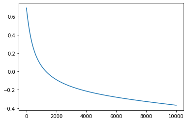
m=gradient_descent_mse(X,Y, epochs=10000, lr=0.01, showw_every=1000)
m

Iteration 0: Error: 0.6931471805599454
Iteration 1000: Error: 0.06119282532013614
Iteration 2000: Error: -0.08993257643349921
Iteration 3000: Error: -0.1657366505381274
Iteration 4000: Error: -0.21517534226106666
Iteration 5000: Error: -0.2518337118318142
Iteration 6000: Error: -0.28128772737254326
Iteration 7000: Error: -0.30637973113973066
Iteration 8000: Error: -0.32875503719447075
Iteration 9000: Error: -0.3494265930621742

array([[0.06737269],
       [1.75403211],
       [1.75409948]])

It seems that our loss is decreasing but is our parameters right? Our bias term should be near to 0 and other parameters should be near to 1 and it can be seen in above case.

Gradient Descent with Logloss’s Gradient

The main reason to use LogLoss is to penalize those which are not performing well.

Derivation of gradient calculated using log loss. \(cost(h_\theta(x),y) = -ylog(h_\theta(x))- (1-y)log(1-h_\theta(x))..(1)\)

From first term, \(log(h_\theta(x)) = log(\frac{1}{1 + e^{-\theta(x)}}) = log(1) - log(1 + e^{-\theta(x)}) = - log(1 + e^{-\theta(x)})\)

From Second term,

\[log(1- h_\theta(x)) = log(1 - \frac{1}{1 + e^{-\theta(x)}}) = log(\frac{e^{-\theta(x)}}{1 + e^{-\theta(x)}}) = log(e^{-\theta(x)}) - log(1 + e^{-\theta(x)}) = -(\theta(x)) - log(1 + e^{-\theta(x)})\]

Do partial derivatives with respect to $\theta$ in (1) \(\frac{1}{d(\theta)}\frac{1}{m}\sum(y.log(1 + e^{-\theta(x)}) +(\theta(x)) +log(1 + e^{-\theta(x)}) - y (\theta(x))-y.log(1 + e^{-\theta(x)})\)

\[= \frac{1}{d(\theta)}\frac{1}{m}\sum(\theta(x) +log(1 + e^{-\theta(x)}) - y (\theta(x))\]

\(= \frac{1}{d(\theta)}\frac{1}{m}\sum(loge^{-\theta(x)} + log(1 + e^{-\theta(x)}) - y (\theta(x))\) \(= \frac{1}{d(\theta)}\frac{1}{m}\sum(log(e^{-\theta(x)} + \frac{e^{\theta(x)}}{e^{-\theta(x)}})- y (\theta(x))\) \(= \frac{1}{d(\theta)}\frac{1}{m}\sum(log(1 + e^{\theta(x)}-y (\theta(x))\) \(= \frac{1}{m}\sum(\frac{x e^{\theta(x)}}{1 + e^{\theta(x)}} - y(x))\) \(= \frac{1}{m} \sum((h\theta(x)- y)x)\)

def gradient_descent_ll(X, Y, epochs=100, lr=0.001, showw_every=100):

    X = X.reshape(-1, X.shape[-1])
    Y = Y.reshape(-1, 1)
    
    m = np.vstack([np.zeros(Y.shape[-1]), np.zeros((X.shape[-1],1))])
    X = np.hstack([np.ones((X.shape[0], 1)), X])
    
    n=len(X)
    errs = []
    for i in range(epochs):
        
        yp = logistic(X, m)
        err = log_loss(Y, yp)
        err = np.mean(err)
        
        tm = np.zeros_like(m)
        for j in range(len(m)):
            grad = np.sum((yp - Y)*np.array(X[:,j]).reshape(n, 1))
            tm[j] = m[j] - (lr / n) * grad
        m = tm
        
        errs.append(err)
        if i% showw_every==0:
            print(f"Iteration {i}: Error: {err}")
    plt.plot(errs)
    plt.show()
    return m

Again, lets use same example as previous.

X = np.arange(0,1000).reshape(-1,2)/1000
Y = X.sum(axis=1)
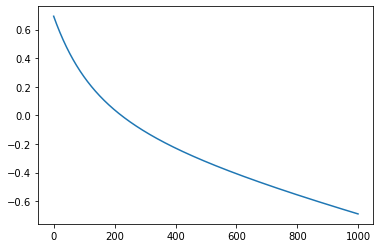
m=gradient_descent_ll(X,Y, epochs=1000, lr=0.01)

Iteration 0: Error: 0.6931471805599454
Iteration 100: Error: 0.2685799686684862
Iteration 200: Error: 0.03779132874320925
Iteration 300: Error: -0.1140519015215765
Iteration 400: Error: -0.22906689034551153
Iteration 500: Error: -0.3244553994714872
Iteration 600: Error: -0.40827659769021674
Iteration 700: Error: -0.48475437370908275
Iteration 800: Error: -0.5563022518074218
Iteration 900: Error: -0.6243944978230606

m

array([[1.44049692],
       [2.22943498],
       [2.23087548]])

The error is decreasing but the parameters are not performing well.

Read csv Data

Here we read Diabetes data which is in csv file formate. In y values we pass Diabetes columns and in x we pass Remaining columns of dataframe. Please find data in kaggle.

df = pd.read_csv("data/Diabetes.csv")

y = df.Diabetes
X = df[[c for c in df.columns if c!="Diabetes"]]
df.head()

	Pragnency	Glucose	Blod Pressure	Skin Thikness	Insulin	BMI	DFP	Age	Diabetes
0	1	85	66	29	0	26.6	0.351	31	0
1	8	183	64	0	0	23.3	0.672	32	1
2	1	89	66	23	94	28.1	0.167	21	0
3	0	137	40	35	168	43.1	2.288	33	1
4	5	116	74	0	0	25.6	0.201	30	0

Split data

Here we split data into train and test set in the proportion of 70% to 30%.

split = int(len(df)*0.7)
train_x, test_x = X[:split].to_numpy() , X[split:].to_numpy()
train_y, test_y = y[:split].to_numpy() , y[split:].to_numpy()

train_x.shape

(536, 8)

Pass our splitted data into the model

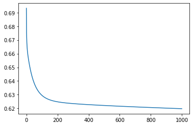
m1=gradient_descent_ll(train_x,train_y, epochs=1000, lr=0.0001)

Iteration 0: Error: 0.6931471805599453
Iteration 100: Error: 0.6295396873352829
Iteration 200: Error: 0.6248296460468838
Iteration 300: Error: 0.6235170017374174
Iteration 400: Error: 0.62275368272634
Iteration 500: Error: 0.622141945309257
Iteration 600: Error: 0.6216012475643053
Iteration 700: Error: 0.6211061190730676
Iteration 800: Error: 0.6206448369613259
Iteration 900: Error: 0.62021069530985

m2 = gradient_descent_mse(train_x,train_y, epochs=1000, lr=0.0001)

Iteration 0: Error: 0.6931471805599453
Iteration 100: Error: 0.6493821418787401
Iteration 200: Error: 0.6393798957706703
Iteration 300: Error: 0.633619122451011
Iteration 400: Error: 0.6301666922801797
Iteration 500: Error: 0.6280087100079533
Iteration 600: Error: 0.6266072658055885
Iteration 700: Error: 0.6256654830359629
Iteration 800: Error: 0.6250123007654729
Iteration 900: Error: 0.6245451868004623

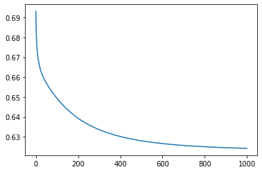
Model error is decreasing.

Function to determine the accuracy of model.

def accuracy(y,yt):
    return np.mean((y.astype(int)==yt.astype(int)).astype(int))

Predict the data

Following predict() function is for making prediction on train as well as untrained data. Here inx = np.hstack([np.ones((x.shape[0], 1)), x]) and x.shape[0] takes only row of data and by using hstack() function we added 1 in each row horizontally as first column. Which is passed into logistic function. The predict function returns: if x is grater than 0.5 result 1 otherwise 0.

def predict(x, m):
    
    x = np.hstack([np.ones((x.shape[0], 1)), x])
    x = logistic(x,m)
    return (x>0.5).astype(np.int)

yp = predict(test_x,m1)

accuracy(predict(test_x,m1),test_y), accuracy(predict(test_x,m2),test_y)

(0.6155994078072, 0.6183354884653586)

Our model accuracy is 61%. Seems that using Logloss to update grads and MSE to update grads is not much difference.

To find precision_score, recall_score, f1_score, accuracy_score

• precision_score : The precision is the ratio tp / (tp + fp) where tp is the number of true positives and fp the number of false positives.
• ` recall_score` : The recall is the ratio tp / (tp + fn) where tp is the number of true positives and fn the number of false negatives
• f1_score: the F-score or F-measure is a measure of a test’s accuracy

from sklearn.metrics import precision_score, recall_score, f1_score, accuracy_score

print(f"Train Accuracy: {accuracy_score(train_y, predict(train_x, m1))}")
print(f"Test Accuracy: {accuracy_score(test_y, predict(test_x, m1))}")

print(f"\nTrain Precision: {precision_score(train_y, predict(train_x, m1))}")
print(f"Test Precision: {precision_score(test_y, predict(test_x, m1))}")

print(f"\nTrain Recall: {recall_score(train_y, predict(train_x, m1))}")
print(f"Test Recall: {recall_score(test_y, predict(test_x, m1))}")

print(f"\nTrain F1: {f1_score(train_y, predict(train_x, m1))}")
print(f"Test F1: {f1_score(test_y, predict(test_x, m1))}")

Train Accuracy: 0.6847014925373134
Test Accuracy: 0.6623376623376623

Train Precision: 0.6
Test Precision: 0.5161290322580645

Train Recall: 0.30319148936170215
Test Recall: 0.20253164556962025

Train F1: 0.40282685512367494
Test F1: 0.2909090909090909

Using Library

from sklearn.linear_model import LogisticRegression

model = LogisticRegression()

model.fit(train_x,train_y)

C:\ProgramData\Anaconda3\lib\site-packages\sklearn\linear_model\_logistic.py:762: ConvergenceWarning: lbfgs failed to converge (status=1):
STOP: TOTAL NO. of ITERATIONS REACHED LIMIT.

Increase the number of iterations (max_iter) or scale the data as shown in:
    https://scikit-learn.org/stable/modules/preprocessing.html
Please also refer to the documentation for alternative solver options:
    https://scikit-learn.org/stable/modules/linear_model.html#logistic-regression
  n_iter_i = _check_optimize_result(





LogisticRegression()

model.intercept_, model.coef_

(array([-7.59822171]),
 array([[ 1.27120498e-01,  3.09123927e-02, -1.00179463e-02,
          8.03188096e-04, -1.19641285e-03,  8.99272976e-02,
          8.13297934e-01,  2.01905173e-03]]))

print(f"Train Accuracy: {accuracy_score(train_y, model.predict(train_x))}")
print(f"Test Accuracy: {accuracy_score(test_y, model.predict(test_x))}")

print(f"\nTrain Precision: {precision_score(train_y, model.predict(train_x))}")
print(f"Test Precision: {precision_score(test_y, model.predict(test_x))}")

print(f"\nTrain Recall: {recall_score(train_y, model.predict(train_x))}")
print(f"Test Recall: {recall_score(test_y, model.predict(test_x))}")

print(f"\nTrain F1: {f1_score(train_y, model.predict(train_x))}")
print(f"Test F1: {f1_score(test_y, model.predict(test_x))}")

Train Accuracy: 0.7742537313432836
Test Accuracy: 0.7922077922077922

Train Precision: 0.7342657342657343
Test Precision: 0.7818181818181819

Train Recall: 0.5585106382978723
Test Recall: 0.5443037974683544

Train F1: 0.634441087613293
Test F1: 0.6417910447761194

Conclusion

• What did we observed while using MSE Gradient?
  • Error was decreasing slowly and its decrease rate was not decreasing.
  • Accuracy was as like log loss.
• What did we observed while using LogLoss Gradient?
  • Error was decreasing fast but its decrease rate was decreasing.
• What did we observed while using Library?
  • Accuracy, F1 Score, Recall and Precision were better.