
Association Rule Mining
Association rule mining, also known as Association Rule Learning, is a popular technique for identifying relationships (or co-occurrences) between multiple variables. It is widely applied in contexts such as grocery stores, e-commerce websites, and other similar establishments to uncover patterns in customer behavior. Additionally, it is highly effective for analyzing massive transactional databases, enabling businesses to optimize inventory, recommend products, and enhance customer experience.
Amazon knows what else you want to buy when you order something on their site. This is a very prevalent example in our daily life. Spotify works on the same principle: they know what song you want to listen to next.
Use of Association Mining Results
Some of most common usages includes:
- Changing the store layout according to trends
- Customer behavior analysis
- Catalogue design
- Cross markteing on online store
- What are the trending items customers buy?
- Customized email with add-on sales
When Association Mining is used?
When we wish to find an association between different objects in a collection, find frequent patterns in a transaction database, relational databases, or any other information repository, we utilize association rule mining. In retailling clustering and classification, association rule mining is found in Marketing Basket Analysis.
By developing a set of rules known as Association Rules, it can tell us what things clients commonly buy together. In simple terms, it generates output in the manner of if this, then that rules.
What is Apriori Algorithm and Rule?
Data from a retail market or an online e-commerce store is typically used to mine association rules. The apriori algorithm makes it easier to detect these patterns or rules rapidly because most transaction data is huge. Using apriori() with all of the rules in the data is not a smart idea!
Rule
- A rule is a note that shows which things are frequently purchased together.
- It has two parts: a ‘LHS’ and a ‘RHS’, which can be represented as follows:
itemssetA => itemssetBis a condition.
Some Association Rule Mining Terms
Support
Association rule are given in the following form,
A=>B[support, confidence]
Where A and B are sets of items in the transaction data. Also, A and B are disjoint sets.
Support = Number of transactions with both A and B / Total number of
transactions = P(A∩B) = frequency(A, B)/N
Confidence
Confidence = Number of transactions with both A and B / Total number of
transactions with A = P(A∩B)/P(A) = frequenc(A, B)/frequency(A)
Expected Confidence
Expected Confidence = Number of transactions withB/Total number of
transactions = P(B) = frequency(B)/N
List
Lift = Confidence/ExpectedConfidence =P(A∩B)/P(A).P(B) =
Support(A,B)/Support(A).Support(B)
Let’s Do Association Rule Mining in R
Create a list of baskets
market_basket<- list(c("bread", "milk"),
                     c("bread","dipers","beer","Egg"),
                     c("milk","dipers","beer","coka"),
                     c("bread","milk","dipers","beer"),
                     c("bread","milk","dipers","coka")
                     )
names(market_basket) <- paste("T",c(1:5),sep = "")
market_basket
## $T1
## [1] "bread" "milk"
##
## $T2
## [1] "bread"  "dipers" "beer"   "Egg"
##
## $T3
## [1] "milk"   "dipers" "beer"   "coka"
##
## $T4
## [1] "bread"  "milk"   "dipers" "beer"
##
## $T5
## [1] "bread"  "milk"   "dipers" "coka"
The five transcations were created from the preceding data and given the names T1,T2,T2,T4,T5.
Now we’ll use the arules package to do some more association rule mining. To move on, we should have installed mention packages.
library(arules)
## Warning: package 'arules' was built under R version 4.1.2

## Loading required package: Matrix

##
## Attaching package: 'arules'

## The following objects are masked from 'package:base':
##
##     abbreviate, write
Let’s make Transformation of transactions.
trans <- as(market_basket,"transactions")
Let’s check dimension of trans variable,
dim(trans)
## [1] 5 6
We received the response 5 6 here, which means we have 5 transactions and 6 products. Let’s take a look at the labels on the objects.
labels(trans)
## [1] "{bread,milk}"             "{beer,bread,dipers,Egg}"
## [3] "{beer,coka,dipers,milk}"  "{beer,bread,dipers,milk}"
## [5] "{bread,coka,dipers,milk}"
Here we got items names we have.
summary(trans)
## transactions as itemMatrix in sparse format with
##  5 rows (elements/itemsets/transactions) and
##  6 columns (items) and a density of 0.6
##
## most frequent items:
##   bread  dipers    milk    beer    coka (Other)
##       4       4       4       3       2       1
##
## element (itemset/transaction) length distribution:
## sizes
## 2 4
## 1 4
##
##    Min. 1st Qu.  Median    Mean 3rd Qu.    Max.
##     2.0     4.0     4.0     3.6     4.0     4.0
##
## includes extended item information - examples:
##   labels
## 1   beer
## 2  bread
## 3   coka
##
## includes extended transaction information - examples:
##   transactionID
## 1            T1
## 2            T2
## 3            T3
Let’s inspect the trans
inspect(trans)
##     items                       transactionID
## [1] {bread, milk}               T1
## [2] {beer, bread, dipers, Egg}  T2
## [3] {beer, coka, dipers, milk}  T3
## [4] {beer, bread, dipers, milk} T4
## [5] {bread, coka, dipers, milk} T5
It is preferable to use the inspect function. It will display ten transactions. In this case, if our data is really huge, a larger number of transaction inspect functions will be necessary.
Relative frequency plot and plot of trans
itemFrequencyPlot(trans, topN=10, cex.names =1)
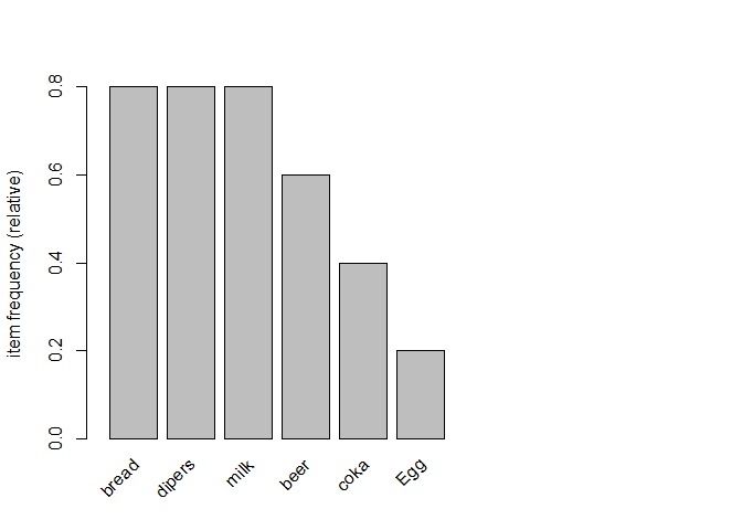
Most sold items were bread, milk and beer similarly less sold item
is Egg.
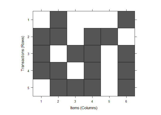
image(trans)
Why Apriori Algorithms is important here?
Because it necessitates a thorough database scan, Frequent Item Set Generation is the most computationally intensive stage. We saw an example of only 5 transactions in the previous example, but real-world transaction data for retail might surpass GBs and TBs of data, necessitating the use of an optimal technique to prune out Item-sets that will not aid in further phases is essential.
Apriori algorithm of “trans” without/with min. support of 0.3 and min. confidence of 0.5.
rues <- apriori(trans)
## Apriori
##
## Parameter specification:
##  confidence minval smax arem  aval originalSupport maxtime support minlen
##         0.8    0.1    1 none FALSE            TRUE       5     0.1      1
##  maxlen target  ext
##      10  rules TRUE
##
## Algorithmic control:
##  filter tree heap memopt load sort verbose
##     0.1 TRUE TRUE  FALSE TRUE    2    TRUE
##
## Absolute minimum support count: 0
##
## set item appearances ...[0 item(s)] done [0.00s].
## set transactions ...[6 item(s), 5 transaction(s)] done [0.00s].
## sorting and recoding items ... [6 item(s)] done [0.00s].
## creating transaction tree ... done [0.00s].
## checking subsets of size 1 2 3 4 done [0.00s].
## writing ... [31 rule(s)] done [0.00s].
## creating S4 object  ... done [0.00s].
rules
## function (rhs, lhs, itemLabels, quality = data.frame())
## {
##     if (!is(lhs, "itemMatrix"))
##         lhs <- encode(lhs, itemLabels = itemLabels)
##     if (!is(rhs, "itemMatrix"))
##         rhs <- encode(rhs, itemLabels = itemLabels)
##     new("rules", lhs = lhs, rhs = rhs, quality = quality)
## }
## <bytecode: 0x0000000022947bd8>
## <environment: namespace:arules>
Here, we made set of 15 rules.
rules <- apriori(trans, parameter = list(supp=0.3,conf=0.5,
                                         maxlen=10,
                                         target ="rules"))
## Apriori
##
## Parameter specification:
##  confidence minval smax arem  aval originalSupport maxtime support minlen
##         0.5    0.1    1 none FALSE            TRUE       5     0.3      1
##  maxlen target  ext
##      10  rules TRUE
##
## Algorithmic control:
##  filter tree heap memopt load sort verbose
##     0.1 TRUE TRUE  FALSE TRUE    2    TRUE
##
## Absolute minimum support count: 1
##
## set item appearances ...[0 item(s)] done [0.00s].
## set transactions ...[6 item(s), 5 transaction(s)] done [0.00s].
## sorting and recoding items ... [5 item(s)] done [0.00s].
## creating transaction tree ... done [0.00s].
## checking subsets of size 1 2 3 done [0.00s].
## writing ... [32 rule(s)] done [0.00s].
## creating S4 object  ... done [0.00s].
Note: maxlen= maximum length of the transaction! We could have used maxlen=4 here as we know it but this will not be known in real-life!
Summary of rules
summary(rules)
## set of 32 rules
##
## rule length distribution (lhs + rhs):sizes
##  1  2  3
##  4 16 12
##
##    Min. 1st Qu.  Median    Mean 3rd Qu.    Max.
##    1.00    2.00    2.00    2.25    3.00    3.00
##
## summary of quality measures:
##     support         confidence        coverage           lift
##  Min.   :0.4000   Min.   :0.5000   Min.   :0.4000   Min.   :0.8333
##  1st Qu.:0.4000   1st Qu.:0.6667   1st Qu.:0.6000   1st Qu.:0.8333
##  Median :0.4000   Median :0.7500   Median :0.6000   Median :1.0000
##  Mean   :0.4938   Mean   :0.7474   Mean   :0.6813   Mean   :1.0473
##  3rd Qu.:0.6000   3rd Qu.:0.8000   3rd Qu.:0.8000   3rd Qu.:1.2500
##  Max.   :0.8000   Max.   :1.0000   Max.   :1.0000   Max.   :1.6667
##      count
##  Min.   :2.000
##  1st Qu.:2.000
##  Median :2.000
##  Mean   :2.469
##  3rd Qu.:3.000
##  Max.   :4.000
##
## mining info:
##   data ntransactions support confidence
##  trans             5     0.3        0.5
##                                                                                            call
##  apriori(data = trans, parameter = list(supp = 0.3, conf = 0.5, maxlen = 10, target = "rules"))
A collection of 32 rules has been created. There are four rules in transaction 1, sixteen in transaction two, and twelve in transaction three. There were also several empty rues generated here. Let’s get rid of these useless rules.
rules <- apriori(trans, parameter = list(supp=0.3,conf = 0.5,
                                         maxlen =10,
                                         minlen=2,
                                         target="rules"))
## Apriori
##
## Parameter specification:
##  confidence minval smax arem  aval originalSupport maxtime support minlen
##         0.5    0.1    1 none FALSE            TRUE       5     0.3      2
##  maxlen target  ext
##      10  rules TRUE
##
## Algorithmic control:
##  filter tree heap memopt load sort verbose
##     0.1 TRUE TRUE  FALSE TRUE    2    TRUE
##
## Absolute minimum support count: 1
##
## set item appearances ...[0 item(s)] done [0.00s].
## set transactions ...[6 item(s), 5 transaction(s)] done [0.00s].
## sorting and recoding items ... [5 item(s)] done [0.00s].
## creating transaction tree ... done [0.00s].
## checking subsets of size 1 2 3 done [0.00s].
## writing ... [28 rule(s)] done [0.00s].
## creating S4 object  ... done [0.00s].
Let’s set RHS rule for trans data
# we set rhs =beer and default = lhs
beer_rules_rhs<- apriori(trans, parameter = list(supp= 0.3,conf= 0.5,
                                                 maxlen= 10,
                                                 minlen=2),
                         appearance = list(default="lhs",
                                           rhs ="beer"))
## Apriori
##
## Parameter specification:
##  confidence minval smax arem  aval originalSupport maxtime support minlen
##         0.5    0.1    1 none FALSE            TRUE       5     0.3      2
##  maxlen target  ext
##      10  rules TRUE
##
## Algorithmic control:
##  filter tree heap memopt load sort verbose
##     0.1 TRUE TRUE  FALSE TRUE    2    TRUE
##
## Absolute minimum support count: 1
##
## set item appearances ...[1 item(s)] done [0.00s].
## set transactions ...[6 item(s), 5 transaction(s)] done [0.00s].
## sorting and recoding items ... [5 item(s)] done [0.00s].
## creating transaction tree ... done [0.00s].
## checking subsets of size 1 2 3 done [0.00s].
## writing ... [5 rule(s)] done [0.00s].
## creating S4 object  ... done [0.00s].
inspect(beer_rules_rhs)
##     lhs                rhs    support confidence coverage lift      count
## [1] {bread}         => {beer} 0.4     0.5000000  0.8      0.8333333 2
## [2] {milk}          => {beer} 0.4     0.5000000  0.8      0.8333333 2
## [3] {dipers}        => {beer} 0.6     0.7500000  0.8      1.2500000 3
## [4] {bread, dipers} => {beer} 0.4     0.6666667  0.6      1.1111111 2
## [5] {dipers, milk}  => {beer} 0.4     0.6666667  0.6      1.1111111 2
People who bought beer said their most recent purchase was dipers, and their most recent sales were breads, dipers, and dipers, as well as milk. It’s a pretty interesting data insight. We can deduce from this that the fathers most likely went to the grocery store to get the baby’s necessities.
Let’s put beer in LHS and set RHS as default values
beer_rules_lhs <- apriori(trans, parameter = list(supp=0.3,conf=0.5,
                                                  maxlen =10,
                                                  minlen =2),
                          appearance = list(default="rhs",lhs ="beer"))
## Apriori
##
## Parameter specification:
##  confidence minval smax arem  aval originalSupport maxtime support minlen
##         0.5    0.1    1 none FALSE            TRUE       5     0.3      2
##  maxlen target  ext
##      10  rules TRUE
##
## Algorithmic control:
##  filter tree heap memopt load sort verbose
##     0.1 TRUE TRUE  FALSE TRUE    2    TRUE
##
## Absolute minimum support count: 1
##
## set item appearances ...[1 item(s)] done [0.00s].
## set transactions ...[6 item(s), 5 transaction(s)] done [0.00s].
## sorting and recoding items ... [5 item(s)] done [0.00s].
## creating transaction tree ... done [0.00s].
## checking subsets of size 1 2 done [0.00s].
## writing ... [3 rule(s)] done [0.00s].
## creating S4 object  ... done [0.00s].
inspect(beer_rules_lhs)
##     lhs       rhs      support confidence coverage lift      count
## [1] {beer} => {bread}  0.4     0.6666667  0.6      0.8333333 2
## [2] {beer} => {milk}   0.4     0.6666667  0.6      0.8333333 2
## [3] {beer} => {dipers} 0.6     1.0000000  0.6      1.2500000 3
People who bought beer would then buy dipers. We can see that the person who buys the most drinks also buys the most diapers.
Product Recommendation Rule
rules_conf<- sort(rules,by ="confidence",
                  decreasing = TRUE)
inspect(rules_conf)
##      lhs                rhs      support confidence coverage lift      count
## [1]  {coka}          => {milk}   0.4     1.0000000  0.4      1.2500000 2
## [2]  {coka}          => {dipers} 0.4     1.0000000  0.4      1.2500000 2
## [3]  {beer}          => {dipers} 0.6     1.0000000  0.6      1.2500000 3
## [4]  {coka, milk}    => {dipers} 0.4     1.0000000  0.4      1.2500000 2
## [5]  {coka, dipers}  => {milk}   0.4     1.0000000  0.4      1.2500000 2
## [6]  {beer, milk}    => {dipers} 0.4     1.0000000  0.4      1.2500000 2
## [7]  {beer, bread}   => {dipers} 0.4     1.0000000  0.4      1.2500000 2
## [8]  {dipers}        => {beer}   0.6     0.7500000  0.8      1.2500000 3
## [9]  {milk}          => {bread}  0.6     0.7500000  0.8      0.9375000 3
## [10] {bread}         => {milk}   0.6     0.7500000  0.8      0.9375000 3
## [11] {milk}          => {dipers} 0.6     0.7500000  0.8      0.9375000 3
## [12] {dipers}        => {milk}   0.6     0.7500000  0.8      0.9375000 3
## [13] {bread}         => {dipers} 0.6     0.7500000  0.8      0.9375000 3
## [14] {dipers}        => {bread}  0.6     0.7500000  0.8      0.9375000 3
## [15] {beer}          => {milk}   0.4     0.6666667  0.6      0.8333333 2
## [16] {beer}          => {bread}  0.4     0.6666667  0.6      0.8333333 2
## [17] {dipers, milk}  => {coka}   0.4     0.6666667  0.6      1.6666667 2
## [18] {beer, dipers}  => {milk}   0.4     0.6666667  0.6      0.8333333 2
## [19] {dipers, milk}  => {beer}   0.4     0.6666667  0.6      1.1111111 2
## [20] {beer, dipers}  => {bread}  0.4     0.6666667  0.6      0.8333333 2
## [21] {bread, dipers} => {beer}   0.4     0.6666667  0.6      1.1111111 2
## [22] {bread, milk}   => {dipers} 0.4     0.6666667  0.6      0.8333333 2
## [23] {dipers, milk}  => {bread}  0.4     0.6666667  0.6      0.8333333 2
## [24] {bread, dipers} => {milk}   0.4     0.6666667  0.6      0.8333333 2
## [25] {milk}          => {coka}   0.4     0.5000000  0.8      1.2500000 2
## [26] {dipers}        => {coka}   0.4     0.5000000  0.8      1.2500000 2
## [27] {milk}          => {beer}   0.4     0.5000000  0.8      0.8333333 2
## [28] {bread}         => {beer}   0.4     0.5000000  0.8      0.8333333 2
The rules are sorted by confidence in decreasing order in the above results.
Plotting rules with “arulesViz” package
library(arulesViz)
## Warning: package 'arulesViz' was built under R version 4.1.2
plot(rules)
## To reduce overplotting, jitter is added! Use jitter = 0 to prevent jitter.
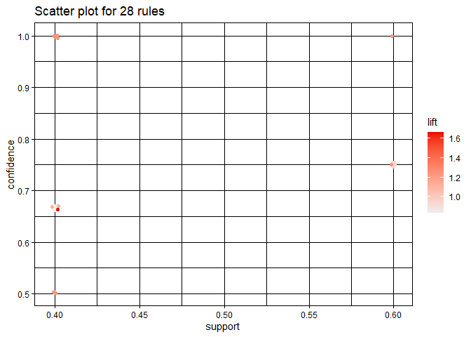
Here, darker orange color indicate those items whose lift value is maximun when lift values decrease colar also become light orange.
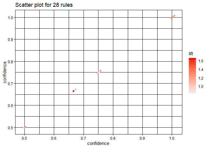
Let’s plot the same plot by setting measure = "confidence".
plot(rules, measure = "confidence")
## To reduce overplotting, jitter is added! Use jitter = 0 to prevent jitter.
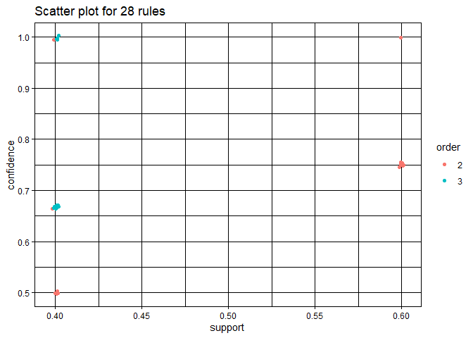
Plot two-key-plot
library(arulesViz)
plot(rules, method = 'two-key plot')
## To reduce overplotting, jitter is added! Use jitter = 0 to prevent jitter.
Plot with “ggplot2” engine
library(ggplot2)

plot(rules, engine = "ggplot2")
## To reduce overplotting, jitter is added! Use jitter = 0 to prevent jitter.

If we hover our curcer above orange points we can see the value of supp, conf as well as left. Darker the orange color more will be the value of corresponing parameters.
Parallel Coordinate plot for 10 rules
plot(subrules, method = "paracoord")
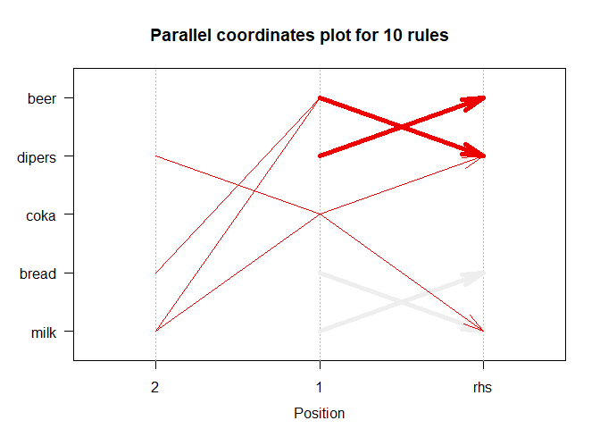
We used the parallel coordinate approach to see in higher-dimensional space. In this case, we visualize in ten dimensions.
Thank you for reading.


Comments