Stock Price Prediction On Commercial Data Using LSTM

Basic Introduction about LSTM

RNNs are unable to remember long-term dependencies in time series data because of the vanishing gradient issue. An RNN version called LSTM was created to deal with this problem. Similar to RNN, LSTM features a hidden state that functions as short-term memory. Additionally, it preserves cell state, which functions as long-term memory.

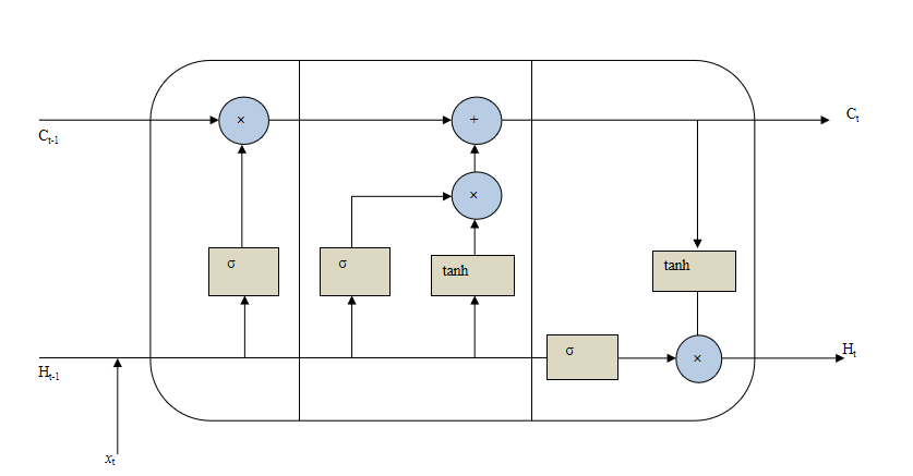
Three gates a forget gate, an input gate, and a output gate make up the LSTM architecture. The forget gate is in place to decide what data from the previous state needs to be remembered and what can be forgotten. Which data from the current input is saved in the cell state depends on the input gate. Finally, the output gate determines the next hidden state value. The LSTM network’s architecture is depicted in the Figure

Import

Here we import necessary module which we required while Fitting LSTM model on Commercial data.

pandas : For data analysis and data manipulation

numpy : for array manipulation and able to work with array type data

matplotlib: For data visualization and analysis of data

cufflinks : for making interactive plot with pandas data

` keras` : to fit LSTM model using keras library

import numpy as np
import pandas as pd
import matplotlib.pyplot as plt
from keras.models import Sequential
from keras.layers import Dense, LSTM
import math
from sklearn.preprocessing import MinMaxScaler,StandardScaler 
from sklearn.model_selection import train_test_split
import cufflinks
cufflinks.go_offline()
cufflinks.set_config_file(world_readable=True, theme='pearl')

Read Data

This specific data is acquired from GitHub, which houses numerous csv files from various businesses. However, I used data from a commercial bank for this LSTM model. There are 2572 rows in all.

#data = "ALICL_2000-01-01_2021-12-31.csv"
commerce = pd.read_csv("ADBL_2000-01-01_2021-12-31.csv", engine='python')
commerce.head()

	S.N.	Date	Total Transactions	Total Traded Shares	Total Traded Amount	Max. Price	Min. Price	Close Price
0	1	2021-12-29	1013	200533.0	98526860.8	499.0	488.0	492.0
1	2	2021-12-28	659	91046.0	44737396.5	498.0	488.0	494.0
2	3	2021-12-27	816	88858.0	44186856.3	510.0	491.0	493.0
3	4	2021-12-26	1002	130801.0	65306688.9	502.0	495.0	500.0
4	5	2021-12-23	714	77234.0	38044401.2	497.0	481.0	496.0

commerce.shape

(2572, 8)

# Sort Data in Ascending order Our data is arranged according to time in descending order. In order to maintain our data in rising order according to our date property, we here change the given data into ascending order. Using the built-in function head, we were able to only examine a portion of the given data set (). We can only access the top 5 data points of the provided dataset by utilizing this head function.

commerce = commerce.sort_values(by="Date")
commerce.head()

	S.N.	Date	Total Transactions	Total Traded Shares	Total Traded Amount	Max. Price	Min. Price	Close Price
2571	2572	2010-08-26	2	40.0	10150.0	255.0	250.0	250.0
2570	2571	2010-08-29	2	20.0	4860.0	245.0	241.0	241.0
2569	2570	2010-08-30	6	60.0	13620.0	237.0	217.0	217.0
2568	2569	2010-08-31	6	60.0	12210.0	213.0	196.0	196.0
2567	2568	2010-09-02	6	60.0	11130.0	193.0	178.0	178.0

Handle Missing NAs

Our analysis might not be successful if there are any missing values. Therefore, we need look for missing values to make our data clean and able to be evaluated. If necessary, we can substitute the missing value with the prior or following value using the average of the other values. However, we ignore the missing data in this instance.

#Handle missing data by dropinig NAs.
commerce = commerce.dropna()
commerce.tail()

	S.N.	Date	Total Transactions	Total Traded Shares	Total Traded Amount	Max. Price	Min. Price	Close Price
4	5	2021-12-23	714	77234.0	38044401.2	497.0	481.0	496.0
3	4	2021-12-26	1002	130801.0	65306688.9	502.0	495.0	500.0
2	3	2021-12-27	816	88858.0	44186856.3	510.0	491.0	493.0
1	2	2021-12-28	659	91046.0	44737396.5	498.0	488.0	494.0
0	1	2021-12-29	1013	200533.0	98526860.8	499.0	488.0	492.0

Plot Trend

Here, we plot our statistics to see how they are trending. by keeping the data in the line plot’s horizontal axis and the closing price in its vertical axis. We are aware that time series data is information that varies over time. As a result, they lack a steady trend.

commerce.iplot(kind="line",x="Date",y="Close Price",xTitle="Date", yTitle="Close Price", title="Commercial Bank Data Trend")

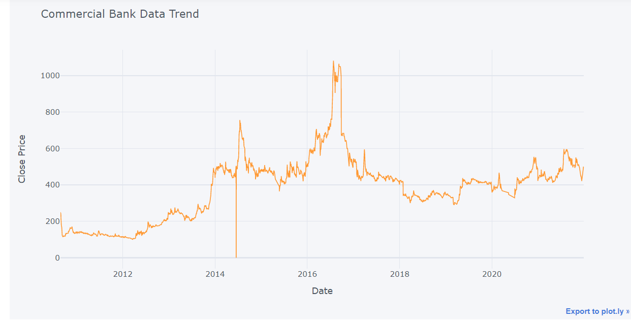
The graph shows that the initial closure price was around 270, and that it subsequently declined before gradually rising to its ideal level in July 2020, which was around 1200. Throughout the remaining time frame, there are frequent changes in closing price.

Next Price

To obtain the next price we shift close price one step back. Because tomorrow closed price is next price for today. And in next step we drop the missing values.

commerce['Next Price'] = commerce.shift(-1)['Close Price']

commerce= commerce.dropna()

Rename Columns

We changed the column names of the provided dataset because some of the original data’s columns weren’t initialized in the typical order; this made various manipulation chores easier.

commerce.rename(columns = {'S.N.':'SN','Total Transactions':'TTrans', 'Total Traded Shares':'TTS',
                              'Total Traded Amount':'TTA','Close Price':'ClosePrice','Next Price':'NextPrice',
                     'Max. Price':'MaxPrice','Min. Price':'MinPrice'}, inplace = True)

Prepared Feature

Here we take Closeprice and Date as a features and NextPrice and Date as outfeature.

features = ['ClosePrice',"Date"]
outFeature = ['NextPrice',"Date"]

Here we assign variable X and Y to the features and outFeasture variable.

# take close price as feature and next price as out feature
X, Y = commerce[features], commerce[outFeature] 
X.set_index("Date", inplace=True)
Y.set_index("Date", inplace=True)

Normalize Data

Here, minmax normalization is used. To alter our data on the same scale, data standardization is increasingly necessary. Data normalization is therefore a crucial stage in the process of converting all data to the same measuring unit.

#Normalize data using standard scalar.
ss = StandardScaler()

X["ClosePrice"] = ss.fit_transform(X)
Y["NextPrice"] = ss.fit_transform(Y)

Train Test Split

Data will be randomly split using train test split of sklearn, losing the sequence. As a result, we created scratch sets for our train and test datasets. We divided the data as follows: we used 80% of the data for the train set, 10% for the validation set, and the final 10% for the test set.

def train_test_split(x,y,train_size):
    n = int(len(x)*train_size)
    trainx = x[:n]
    testx = x[n:]
    trainy=y[:n]
    testy=y[n:]
    return trainx,testx,trainy,testy

#Split train, validation, test set from X,Y to 80%, 10%, 10%

X_train, X_test, Y_train, Y_test = train_test_split(X, Y, train_size=0.9)

X_train.shape,X_test.shape,X.shape

((2313, 1), (258, 1), (2571, 1))

Here, we divided our data into five-sequence groupings. We used the first five pieces of data in the first series. We kept the first data in the second sequence and added six more. In the third sequence, we left the second sequence alone and added seven new data points. The sequence selection procedure was carried out in this manner. We took 25 hidden layers from this hidden layer. We also used 50 layers for the input and output layers.

model = Sequential()
model.add(LSTM(units=50, return_sequences=True,input_shape=(5,1)))
model.add(LSTM(units=50, return_sequences=False))
model.add(Dense(units=25))
model.add(Dense(units=1))

Convert to matrix

Here, we convert train, test set of data into matrix inorder to do calculation easy.

# convert into dataset matrix
def convertToMatrix(data, step):
    data = data.to_numpy()
    X, Y =[], []
    for i in range(len(data)-step):
        d=i+step  
        X.append(data[i:d,])
        Y.append(data[d,])
    return np.array(X), np.array(Y)

step=5

trainX,trainY =convertToMatrix(X_train,step)
testX,testY =convertToMatrix(X_test,step)
# validX,validY = convertToMatrix(X_valid,step)

trainX = np.reshape(trainX, (trainX.shape[0], trainX.shape[1],1))
# validX = np.reshape(validX, (validX.shape[0], 1, validX.shape[1]))
testX = np.reshape(testX, (testX.shape[0], testX.shape[1],1))

trainX.shape,testX.shape #,validX.shape

((2308, 5, 1), (253, 5, 1))

We perform model compilation in the code below. Here, we used mean squared error as the loss function and the Adam optimizer as our optimization function. Next, we fitted the model using the train, test, batch size, and epochs parameters. We finally received a loss of 0.0358.

model.compile(optimizer='adam', loss='mean_squared_error')
model.fit(trainX, trainY, batch_size=1, epochs=1)

2308/2308 [==============================] - 13s 4ms/step - loss: 0.0389





<keras.callbacks.History at 0x27d130762b0>

In the following block of the code we perform model prediction operation.

predictions = model.predict(testX)
predictions = ss.inverse_transform(predictions)
predictions.shape,testX.shape

8/8 [==============================] - 1s 4ms/step





((253, 1), (253, 5, 1))

From this model we get RMSE value 13.58. We know that we expect lower value of RMSE as possible.

Y_test_ss = ss.inverse_transform(Y_test)[:-5]

rmse=np.sqrt(np.mean(((predictions- Y_test_ss)**2)))
print(rmse)

27.81754085685057

Test Trend

test=pd.DataFrame()
test["pred"]=ss.inverse_transform(predictions.flatten())
test["real"]=ss.inverse_transform(Y_test_ss)
test["date"]=X_test.index[:-5]
test.iplot(kind="line", x="date",xTitle ="Date",yTitle= "Closed Price",title= "Trend of Closed Price")

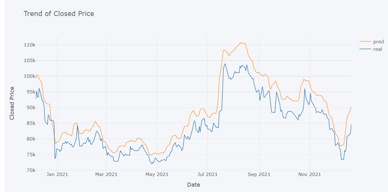
The test trend of our data is depicted in the following graphs. The numbers show that the test trend differs in some way from the data’s original trend. Here, the blue hue represents the actual trend of the data, while the orange color represents the forecast trend. We can tell from the figures that our model is overfitting. The model predicts the best price on July 22, 2021, but on other days it anticipates erratic price movements.